New Features in Maple 2018 - Advanced Math - Maplesoft

What's New in Maple 2018

Advanced Math

In addition to the mathematical advances detailed in other sections, Maple 2018 also includes improvements across many other areas of the mathematics engine.


Integration

The int command has seen improvements to various methods. The following new results come from the asymptotic method:

int(`/`(`*`(sin(x)), `*`(`^`(x, 3))), x = 0 .. infinity)
infinity

int(`/`(`*`(cos(x), `*`(cos(`+`(`*`(`/`(1, 3), `*`(x)))))), `*`(`^`(x, 2))), x = 0 .. infinity)
infinity

This new result results from an improvement in the elliptic integration code:

int(abs(`+`(exp(`*`(`*`(2, `*`(I)), `*`(Pi, `*`(x)))), exp(`*`(`*`(2, `*`(I)), `*`(Pi, `*`(y)))))), [x = 0 .. 1, y = 0 .. 1])
`+`(`/`(`*`(4), `*`(Pi)))

The next two examples are due to improvements to the Risch algorithm: normal(int(`/`(`*`(sin(`*`(x, `*`(arctan(a)))), `*`(`^`(`+`(`*`(`^`(a, 2)), 1), `+`(`-`(x))))), `*`(`+`(1, exp(a)))), x))

`+`(`-`(`/`(`*`(exp(`+`(`-`(`*`(x, `*`(ln(`+`(`*`(`^`(a, 2)), 1))))))), `*`(`+`(`-`(`*`(arctan(a), `*`(`^`(tan(`+`(`*`(`/`(1, 2), `*`(x, `*`(arctan(a)))))), 2)))), `*`(2, `*`(ln(`+`(`*`(`^`(a, 2)), 1)...

int(`+`(`*`(`+`(`*`(`/`(83, 30), `*`(`^`(ln(u), 2))), `-`(`*`(`/`(20162, 2025), `*`(ln(u)))), `/`(584972, 30375)), `*`(`^`(u, `/`(5, 2)))), `*`(`+`(`*`(`/`(4723, 1260), `*`(`^`(ln(u), 2))), `-`(`*`(`/...
`+`(`*`(`/`(83, 105), `*`(`^`(u, `/`(7, 2)), `*`(`^`(ln(u), 2)))), `-`(`*`(`/`(327088, 99225), `*`(`^`(u, `/`(7, 2)), `*`(ln(u))))), `*`(`/`(67139896, 10418625), `*`(`^`(u, `/`(7, 2)))), `*`(`/`(4723,...

This previously unsolved example is due to an improvement in the hyperexponential algorithm:


int(`/`(`*`(sqrt(`+`(sinh(x), cosh(x)))), `*`(`+`(sinh(x), 1))), x)
`+`(`-`(`/`(`*`(`/`(1, 2), `*`(`^`(`+`(`-`(`/`(`*`(`+`(tanh(`+`(`*`(`/`(1, 2), `*`(x)))), 1)), `*`(`+`(tanh(`+`(`*`(`/`(1, 2), `*`(x)))), `-`(1)))))), `/`(1, 2)), `*`(`+`(tanh(`+`(`*`(`/`(1, 2), `*`(x...

Simplification

The simplify command has been enhanced with respect to logarithms whose arguments are constant radical expressions. Some examples:

simplify(`+`(ln(`+`(1, `-`(sqrt(2)))), ln(`+`(1, sqrt(2)))))
`*`(I, `*`(Pi))

simplify(ln(`+`(sqrt(`+`(2, sqrt(2))), sqrt(`+`(`-`(2), sqrt(2))))))
`+`(ln(2), `*`(`*`(`/`(1, 8), `*`(I)), `*`(Pi)))

simplify(`+`(`-`(`*`(7, `*`(Pi, `*`(ln(`+`(2, `-`(sqrt(3)))))))), `*`(11, `*`(Pi, `*`(ln(`+`(2, sqrt(3)))))), `*`(38, `*`(ln(`+`(sqrt(3), `-`(1))), `*`(Pi))), `*`(2, `*`(Pi, `*`(ln(`+`(1, sqrt(3))))))...
`+`(`*`(24, `*`(Pi, `*`(ln(2)))))

simplify can now recognize more trig and exp simplifications:
simplify(`+`(`-`(cos(`+`(`*`(`/`(1, 12), `*`(Pi))))), sin(`+`(`*`(`/`(1, 12), `*`(Pi)))), `*`(`/`(1, 2), `*`(sqrt(2)))))

0

simplify(`+`(`*`(16, `*`(sin(`+`(`*`(`/`(4, 9), `*`(Pi)))))), `-`(`*`(24, `*`(sin(`+`(`*`(`/`(1, 9), `*`(Pi))))))), `-`(`*`(32, `*`(sin(`+`(`*`(`/`(2, 9), `*`(Pi))))))), `*`(8, `*`(sqrt(3), `*`(cos(`+...
0

simplify(`*`(exp(`*`(`*`(`/`(1, 5), `*`(I)), `*`(Pi))), `*`(`+`(`*`(`/`(1, 4), `*`(sqrt(5))), `/`(1, 4), `-`(`*`(`+`(`*`(`/`(1, 4), `*`(I))), `*`(sqrt(2), `*`(sqrt(`+`(5, `-`(sqrt(5))))))))))))
1

simplify now tries harder to simplify constants that appear as subexpressions:

simplify(`*`(`+`(`*`(`^`(-1, `/`(1, 5))), `-`(`*`(`^`(-1, `/`(2, 5)))), `*`(`^`(-1, `/`(3, 5))), `-`(`*`(`^`(-1, `/`(4, 5)))), `-`(1)), `*`(x)))
0

PolynomialTools

Two new commands, Homogenize and IsHomogeneous, for performing and testing (weighted) homogenization were added to the PolynomialTools package.

with(PolynomialTools); -1
f := `+`(`*`(`^`(w, 5)), `*`(`^`(w, 2), `*`(x)), `*`(`^`(y, 3)), `*`(w, `*`(y)))
Typesetting:-mprintslash([f := `+`(`*`(`^`(w, 5)), `*`(`^`(w, 2), `*`(x)), `*`(`^`(y, 3)), `*`(w, `*`(y)))], [`+`(`*`(`^`(w, 5)), `*`(`^`(w, 2), `*`(x)), `*`(`^`(y, 3)), `*`(w, `*`(y)))])

IsHomogeneous(f)
false

g := Homogenize(f, z)
Typesetting:-mprintslash([g := `+`(`*`(`^`(w, 5)), `*`(`^`(w, 2), `*`(x, `*`(`^`(z, 2)))), `*`(w, `*`(y, `*`(`^`(z, 3)))), `*`(`^`(y, 3), `*`(`^`(z, 2))))], [`+`(`*`(`^`(w, 5)), `*`(`^`(w, 2), `*`(x, ...

IsHomogeneous(g)
true

Homogenize(f, z, [w, x], [1, 2])
`+`(`*`(`^`(y, 3), `*`(`^`(z, 5))), `*`(w, `*`(y, `*`(`^`(z, 4)))), `*`(`^`(w, 5)), `*`(`^`(w, 2), `*`(x, `*`(z))))

Summation

The sum command with the parametric option has been improved for the case of hypergeometric sums with more than one parameter. The following sums used to return unevaluated in Maple 2017.

sum(`/`(`*`(`^`(x, n)), `*`(`+`(n, b))), n = 0 .. infinity, parametric)
Typesetting:-mprintslash([PIECEWISE([FAIL, b = 0], [`/`(1, `*`(b)), And(x = 0, `<>`(b, 0))], [PIECEWISE([FAIL, (`+`(1, b))::nonposint], [LerchPhi(x, 1, b), And(`<=`(abs(x), 1), `<>`(x, 1), (`+`(1, b))...

sum(`*`(binomial(`+`(i, k, `-`(1)), i), `*`(`^`(z, i))), i = 0 .. infinity, parametric)

Typesetting:-mprintslash([PIECEWISE([`/`(1, `*`(`^`(`+`(1, `-`(z)), k))), Or(k::nonposint, And(abs(z) = 1, `<`(0, `+`(`-`(Re(k))))), And(abs(z) = 1, `<>`(z, 1), `<`(-1, `+`(`-`(Re(k)))), `<=`(`+`(`-`(...

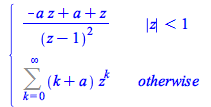
sum(`*`(`+`(k, a), `*`(`^`(z, k))), k = 0 .. infinity, parametric)
piecewise(`<`(abs(z), 1), `/`(`*`(`+`(`-`(`*`(a, `*`(z))), a, z)), `*`(`^`(`+`(z, `-`(1)), 2))), Sum(`*`(`+`(k, a), `*`(`^`(z, k))), k = 0 .. infinity))

Sturm Sequences

The commands sturm and sturmseq have been extended to support polynomials with real algebraic number coefficients.
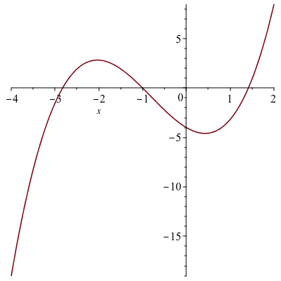
f := expand(`*`(`+`(x, `-`(sqrt(2))), `*`(`+`(x, 1), `*`(`+`(x, `*`(2, `*`(sqrt(2))))))))
Typesetting:-mprintslash([f := `+`(`*`(`^`(x, 3)), `*`(`^`(x, 2), `*`(`^`(2, `/`(1, 2)))), `*`(`^`(x, 2)), `*`(`^`(2, `/`(1, 2)), `*`(x)), `-`(`*`(4, `*`(x))), `-`(4))], [`+`(`*`(`^`(x, 3)), `*`(`^`(x...

s := sturmseq(f, x)
Typesetting:-mprintslash([s := [`+`(`*`(`^`(x, 3)), `*`(`^`(x, 2), `*`(`^`(2, `/`(1, 2)))), `*`(`^`(x, 2)), `*`(`^`(2, `/`(1, 2)), `*`(x)), `-`(`*`(4, `*`(x))), `-`(4)), `+`(`*`(`^`(x, 2)), `*`(`/`(2,...

sturm(s, x = `+`(`-`(infinity)) .. 0)
2

sturm(s, x = 0 .. 5)
1

plot(f, x = -4 .. 2)
Plot_2d

signum

The signum command has had various improvements made. The following examples previously returned with unevaluated signum calls:

`assuming`([`~`[signum]([`^`(-1, x), `^`(I, x)])], [x::real])
[`^`(-1, x), `^`(I, x)]

`assuming`([`~`[signum]([`^`(I, `+`(`*`(2, `*`(x)))), `^`(I, `+`(`*`(2, `*`(x)), 1))])], [x::even])
[1, I]

`assuming`([`~`[signum]([`^`(I, `+`(`*`(2, `*`(x)))), `^`(I, `+`(`*`(2, `*`(x)), 1))])], [x::odd])
[-1, `+`(`-`(I))]

signum(sqrt(`+`(`-`(`/`(`*`(6, `*`(`+`(`*`(sqrt(`/`(`*`(`+`(`*`(`^`(`+`(108, `*`(`*`(12, `*`(I)), `*`(sqrt(687)))), `/`(2, 3))), 48)), `*`(`^`(`+`(108, `*`(`*`(12, `*`(I)), `*`(sqrt(687)))), `/`(1, 3)...
I

is, coulditbe

The is and coulditbe commands have had various improvements made. is performs more simplification than it did previously:

is(`*`(exp(1), `*`(exp(-1))), integer)
true

`assuming`([is(`>`(`+`(`-`(`*`(`+`(I), `*`(`^`(I, `+`(`*`(2, `*`(n)), 1)))))), 0))], [n::even])
true

and takes into account more function properties:

`assuming`([is(`>=`(`+`(arccosh(x), `-`(`*`(`+`(I), `*`(Pi)))), 0))], [`<`(x, -1)])
true

and operation properties:


`assuming`([is(`^`(z, n), imaginary)], [z::imaginary, n::integer, (`^`(z, n))::(Non(real))])
true

The internal solver for systems of inequalities in is and coulditbe has been improved:

`assuming`([map2(coulditbe, p, [-1, 1])], [`<`(-1, p), `<`(-1, q), `<`(-1, r), `<`(-1, `+`(p, q)), `<`(-1, `+`(p, r)), `<`(-1, `+`(r, q)), `<`(-1, `+`(p, q, r))])
[false, true]

Re, Im

The Re and Im commands have had various improvements made. The following examples previously returned with unevaluated Re and Im calls:

`assuming`([Im(z1)], [`>`(z, 0), `<`(z, 1), z1 = arccosh(z)])
`+`(`-`(`*`(`+`(I), `*`(z1))))

([Re, Im])(`*`(I, `*`(GAMMA(`+`(`/`(3, 2), `-`(`*`(`+`(`*`(`/`(1, 2), `*`(I))), `*`(sqrt(3)))))), `*`(GAMMA(`+`(`/`(3, 2), `*`(`*`(`/`(1, 2), `*`(I)), `*`(sqrt(3)))))))))
[0, `*`(GAMMA(`+`(`/`(3, 2), `-`(`*`(`+`(`*`(`/`(1, 2), `*`(I))), `*`(`^`(3, `/`(1, 2))))))), `*`(GAMMA(`+`(`/`(3, 2), `*`(`*`(`/`(1, 2), `*`(I)), `*`(`^`(3, `/`(1, 2))))))))]

max, min

In some cases, the max and min commands can now recognize numbers as real even though they are composed from nonreal ingredients:

max(1, `+`(`*`(`/`(1, 2), `*`(`^`(`+`(`-`(4), `*`(`*`(4, `*`(I)), `*`(sqrt(3)))), `/`(1, 3)))), `/`(`*`(2), `*`(`^`(`+`(`-`(4), `*`(`*`(4, `*`(I)), `*`(sqrt(3)))), `/`(1, 3))))))
`+`(`*`(`/`(1, 2), `*`(`^`(`+`(`-`(4), `*`(`*`(4, `*`(I)), `*`(`^`(3, `/`(1, 2))))), `/`(1, 3)))), `/`(`*`(2), `*`(`^`(`+`(`-`(4), `*`(`*`(4, `*`(I)), `*`(`^`(3, `/`(1, 2))))), `/`(1, 3)))))

evalc(%)
`+`(`*`(2, `*`(cos(`+`(`*`(`/`(2, 9), `*`(Pi)))))))

evalf(%); 1
1.532088886

arctan

The arctan command now performs some more automatic simplifications:

`assuming`([arctan(`/`(`*`(`+`(b, sqrt(`+`(`*`(`^`(a, 2)), `*`(`^`(b, 2)))))), `*`(a)))], [`>`(a, 0), `>`(b, 0)])
`+`(`-`(`*`(`/`(1, 2), `*`(arctan(`/`(`*`(a), `*`(b)))))), `*`(`/`(1, 2), `*`(Pi)))

`assuming`([arctan(`+`(t, sqrt(`+`(`*`(`^`(t, 2)), 1))))], [`>`(t, 0)])
`+`(`-`(`*`(`/`(1, 2), `*`(arctan(`/`(1, `*`(t)))))), `*`(`/`(1, 2), `*`(Pi)))

arctan(`/`(`*`(`+`(`-`(1), sqrt(`+`(`*`(`^`(z, 2)), 1)))), `*`(z)))
`+`(`*`(`/`(1, 2), `*`(arctan(z))))

Furthermore, combine performs more simplifications on arctan functions:

combine(`+`(arctan(`/`(1, `*`(z))), arctan(z)))
`+`(`*`(`/`(1, 2), `*`(csgn(`/`(`*`(`+`(`*`(`^`(z, 2)), 1)), `*`(z))), `*`(Pi))))

`assuming`([combine(expand(`+`(`/`(`*`(arctan(b)), `*`(Pi)), `-`(`/`(`*`(2, `*`(arctan(`+`(b, sqrt(`+`(`*`(`^`(b, 2)), 1)))))), `*`(Pi))))))], [`<`(0, b)])
-`/`(1, 2)

SMTLIB

The SMTLIB package has been extended to support satisfiability queries on Boolean combinations of polynomial equations and inequalities.

Consider the following description of a set: sys := Or(Or(And(And(`<=`(0, `+`(`*`(`^`(y, 2)), x)), `<`(`+`(`*`(`/`(2, 3), `*`(x)), `-`(3)), `+`(`*`(2, `*`(y))))), `<`(y, `+`(`*`(`/`(1, 3), `*`(x)), 1))), And(And(`<`(1, y), `<`(0, `+`(x, y, `-`(1...We can use first use SMTLIB[Satisfiable] to verify that a solution exists:

SMTLIB[Satisfiable](sys)
true

In this simple two-dimensional case, we can use plots[inequal] to visualize the solution space:

with(plots); -1inequal(sys, x = -5 .. 5, y = -5 .. 5)
Plot_2d

The new command SMTLIB[Satisfy] offers an efficient method of finding a concrete example for a point in the solution space:

SMTLIB[Satisfy](sys)
{x = 6, y = 217}

To produce a satisfying point within the visual bounds of the plot above, we can simply augment our system with a bounding rectangle:
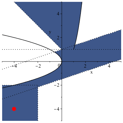
pt := SMTLIB[Satisfy](`and`(`and`(`and`(`and`(sys, `>`(x, -5)), `<`(x, 5)), `>`(y, -5)), `<`(y, 5)))
{x = -4, y = -4}

display(inequal(sys, x = -5 .. 5, y = -5 .. 5), pointplot([eval([x, y], pt)], symbol = solidcircle, symbolsize = 25, color = red)); 1
Plot_2d

Generalized polylogarithms

The GeneralizedPolylog, MultiPolylog and MultiZeta functions have been added to the Maple library, as part of on-going work in the area of mathematical functions.

Generalized polylogarithms [1, 2] (also known as Goncharov polylogarithms, generalized harmonic polylogarithms, or hyperlogarithms) are a class of functions that frequently show up in results for Feynman integrals, as they appear in high energy physics (for overview articles, see e.g. refs. [3, 4]). Therefore tools for their manipulation and evaluation are of high importance for precise predictions in high energy particle scattering processes, as they take place for instance at the Large Hadron Collider at CERN.

Generalized polylogarithms are also a generalization of functions such as the logarithm, the classical (or Euler) polylogarithm, and the harmonic polylogarithm [5], which all appear as special cases.

When evaluated at certain special values, generalized polylogarithms reduce to a set of numbers called multiple zeta values [6, 7, 8], which are a generalization of the values of the Riemann zeta function evaluated at positive integers. Aside form their appearance in physics, these numbers are also of interest in pure mathematics such as number theory.

The generalized polylogarithm is defined recursively, as the iterated integral

GeneralizedPolylog([`$`(a[i], `=`(i, 1 .. w))], x) = %int(`/`(GeneralizedPolylog([`$`(a[i], `=`(i, 2 .. w))], y), `-`(y, a[1])), `=`(y, 0 .. x)) 


The recursion stops, as  


GeneralizedPolylog([], x) = 1 


For all the a[i] indices being zero, an alternative definition is used, as  


GeneralizedPolylog([`$`(0, w)], x) = `/`(`*`(`^`(ln(x), n)), `*`(factorial(n))) 


The multiple polylogarithm, on the other hand, represent the sum form over  


MultiPolylog(`$`(m[i], `=`(i, 1 .. n)), `$`(z[i], `=`(i, 1 .. n))) = %sum(Multiply(`$`(`/`(`^`(z[j], i[j]), `^`(i[j], m[j])), `=`(j, 1 .. n))), i) 


and the analytic continuation thereof outside its convergent region, which is given by the restrictions  


product(a[j], j = 1 .. n) 


`<`(abs(z[1]), 1), `<`(abs(`*`(z[1], `*`(z[2]))), 1), () .. (), `<`(abs(%product(z[i], `=`(i, 1 .. n))), 1) 


MultiZeta is an implementation of multiple zeta values, also known as the generalized Euler sums over


MultiZeta(`$`(m[i], `=`(i, 1 .. n))) = %sum(Multiply(`$`(`/`(1, `^`(i[j], m[j])), `=`(j, 1 .. n))), i)


The sum converges for all positive integer arguments, except when the first argument equals one, for instance as in MultiZeta(1, 2, 3), in which case the function diverges.  


To display special functions using textbook notation, use extended typesetting and enable the typesetting of mathematical functions.

> interface(typesetting = extended); -1; Typesetting:-EnableTypesetRule(Typesetting:-SpecialFunctionRules); -1


Functions such as ln, polylog and MultiZeta may appear as special cases of the generalized polylogarithms  


> %GeneralizedPolylog([0], x) = GeneralizedPolylog([0], x); 1


%GeneralizedPolylog([0], x) = ln(x)

> %GeneralizedPolylog([0, 0, 0, 0, 1], x) = GeneralizedPolylog([0, 0, 0, 0, 1], x); 1


%GeneralizedPolylog([0, 0, 0, 0, 1], x) = `+`(`-`(polylog(5, x)))

Likewise, and using a more compact input syntax

> (%MultiPolylog = MultiPolylog)([2, 3, 4, 5], [1, 1, 1, 1]); 1


%MultiPolylog([2, 3, 4, 5], [1, 1, 1, 1]) = MultiZeta(2, 3, 4, 5)

The Multiple Polylogarithm has been implemented for certain special values such as the oscillating multiple Zeta values up to weight four


> (%MultiPolylog = MultiPolylog)([2, 1, 1], [1, -1, -1])


%MultiPolylog([2, 1, 1], [1, -1, -1]) = `+`(`*`(`/`(1, 8), `*`(`^`(ln(2), 2), `*`(`^`(Pi, 2)))), `-`(`*`(`/`(7, 288), `*`(`^`(Pi, 4)))), `*`(3, `*`(polylog(4, `/`(1, 2)))), `*`(`/`(1, 8), `*`(`^`(ln(2...

and also for certain cases at weights two an three where it reduces directly to classical polylogarithms


> (%MultiPolylog = MultiPolylog)([2, 1], [1, x])


%MultiPolylog([2, 1], [1, x]) = `+`(`*`(polylog(2, `+`(1, `-`(x))), `*`(ln(`+`(1, `-`(x))))), `-`(polylog(3, x)), `-`(`*`(2, `*`(polylog(3, `+`(1, `-`(x)))))), `*`(2, `*`(Zeta(3))))

Similar relations are implemented for the generalized polylogarithm


> (%GeneralizedPolylog = GeneralizedPolylog)([0, 1, 1], x)


%GeneralizedPolylog([0, 1, 1], x) = `+`(`-`(polylog(3, `+`(1, `-`(x)))), `*`(polylog(2, `+`(1, `-`(x))), `*`(ln(`+`(1, `-`(x))))), `*`(`/`(1, 2), `*`(ln(x), `*`(`^`(ln(`+`(1, `-`(x))), 2)))), Zeta(3))

Many relations are obeyed by the generalized polylogarithm, such as the rescaling relation


> GeneralizedPolylog([`+`(.23, `-`(`*`(1.78, `*`(I)))), `+`(1.99, `*`(3.33, `*`(I))), `+`(.77, `*`(0.9e-1, `*`(I)))], `+`(1.35, `-`(`*`(1.01, `*`(I)))))


GeneralizedPolylog([`+`(.23, `-`(`*`(1.78, `*`(I)))), `+`(1.99, `*`(3.33, `*`(I))), `+`(.77, `*`(0.9e-1, `*`(I)))], `+`(1.35, `-`(`*`(1.01, `*`(I)))))

> GeneralizedPolylog([`*`(`+`(.23, `-`(`*`(1.78, `*`(I)))), `*`(z)), `*`(`+`(1.99, `*`(3.33, `*`(I))), `*`(z)), `*`(`+`(.77, `*`(0.9e-1, `*`(I))), `*`(z))], `*`(`+`(1.35, `-`(`*`(1.01, `*`(I)))), `*`(z)...


GeneralizedPolylog([`*`(`+`(.23, `-`(`*`(1.78, `*`(I)))), `*`(z)), `*`(`+`(1.99, `*`(3.33, `*`(I))), `*`(z)), `*`(`+`(.77, `*`(0.9e-1, `*`(I))), `*`(z))], `*`(`+`(1.35, `-`(`*`(1.01, `*`(I)))), `*`(z)...

Evaluate numerically GeneralizedPolylog([`+`(.23, `-`(`*`(1.78, `*`(I)))), `+`(1.99, `*`(3.33, `*`(I))), `+`(.77, `*`(0.9e-1, `*`(I)))], `+`(1.35, `-`(`*`(1.01, `*`(I))))) and GeneralizedPolylog([`*`(`+`(.23, `-`(`*`(1.78, `*`(I)))), `*`(z)), `*`(`+`(1.99, `*`(3.33, `*`(I))), `*`(z)), `*`(`+`(.77, `*`(0.9e-1, `*`(I))), `*`(z))], `*`(`+`(1.35, `-`(`*`(1.01, `*`(I)))), `*`(z)... up to 8 digits

> evalf[8](eval(GeneralizedPolylog([`+`(.23, `-`(`*`(1.78, `*`(I)))), `+`(1.99, `*`(3.33, `*`(I))), `+`(.77, `*`(0.9e-1, `*`(I)))], `+`(1.35, `-`(`*`(1.01, `*`(I))))) = GeneralizedPolylog([`*`(`+`(.23, ...
evalf[8](eval(GeneralizedPolylog([`+`(.23, `-`(`*`(1.78, `*`(I)))), `+`(1.99, `*`(3.33, `*`(I))), `+`(.77, `*`(0.9e-1, `*`(I)))], `+`(1.35, `-`(`*`(1.01, `*`(I))))) = GeneralizedPolylog([`*`(`+`(.23, ...


`+`(0.13040566e-1, `*`(.21053300, `*`(I))) = `+`(0.13040566e-1, `*`(.21053300, `*`(I)))

and the shuffle relation


> `*`(GeneralizedPolylog([`+`(.23, `-`(`*`(1.78, `*`(I))))], `+`(1.35, `-`(`*`(1.01, `*`(I))))), `*`(GeneralizedPolylog([`+`(1.99, `*`(3.33, `*`(I))), `+`(.77, `*`(0.9e-1, `*`(I)))], `+`(1.35, `-`(`*`(1...


`*`(`+`(`-`(.2780299456), `-`(`*`(1.097010462, `*`(I)))), `*`(GeneralizedPolylog([`+`(1.99, `*`(3.33, `*`(I))), `+`(.77, `*`(0.9e-1, `*`(I)))], `+`(1.35, `-`(`*`(1.01, `*`(I)))))))

> `+`(GeneralizedPolylog([`+`(.23, `-`(`*`(1.78, `*`(I)))), `+`(1.99, `*`(3.33, `*`(I))), `+`(.77, `*`(0.9e-1, `*`(I)))], `+`(1.35, `-`(`*`(1.01, `*`(I))))), GeneralizedPolylog([`+`(1.99, `*`(3.33, `*`(...
`+`(GeneralizedPolylog([`+`(.23, `-`(`*`(1.78, `*`(I)))), `+`(1.99, `*`(3.33, `*`(I))), `+`(.77, `*`(0.9e-1, `*`(I)))], `+`(1.35, `-`(`*`(1.01, `*`(I))))), GeneralizedPolylog([`+`(1.99, `*`(3.33, `*`(...
 

`+`(GeneralizedPolylog([`+`(.23, `-`(`*`(1.78, `*`(I)))), `+`(1.99, `*`(3.33, `*`(I))), `+`(.77, `*`(0.9e-1, `*`(I)))], `+`(1.35, `-`(`*`(1.01, `*`(I))))), GeneralizedPolylog([`+`(1.99, `*`(3.33, `*`(...

Up to 6 digits,

> evalf[6](`*`(`+`(`-`(.2780299456), `-`(`*`(1.097010462, `*`(I)))), `*`(GeneralizedPolylog([`+`(1.99, `*`(3.33, `*`(I))), `+`(.77, `*`(0.9e-1, `*`(I)))], `+`(1.35, `-`(`*`(1.01, `*`(I))))))) = `+`(Gene...


and the "stuffle" relation


> `*`(%MultiPolylog([2], [`+`(.98, `-`(`*`(.11, `*`(I))))]), `*`(%MultiPolylog([3], [`+`(2.77, `-`(`*`(1.04, `*`(I))))])))


`*`(%MultiPolylog([2], [`+`(.98, `-`(`*`(.11, `*`(I))))]), `*`(%MultiPolylog([3], [`+`(2.77, `-`(`*`(1.04, `*`(I))))])))

> `+`(%MultiPolylog([2, 3], [`+`(.98, `-`(`*`(.11, `*`(I)))), `+`(2.77, `-`(`*`(1.04, `*`(I))))]), %MultiPolylog([3, 2], [`+`(2.77, `-`(`*`(1.04, `*`(I)))), `+`(.98, `-`(`*`(.11, `*`(I))))]), %MultiPoly...
`+`(%MultiPolylog([2, 3], [`+`(.98, `-`(`*`(.11, `*`(I)))), `+`(2.77, `-`(`*`(1.04, `*`(I))))]), %MultiPolylog([3, 2], [`+`(2.77, `-`(`*`(1.04, `*`(I)))), `+`(.98, `-`(`*`(.11, `*`(I))))]), %MultiPoly...


`+`(%MultiPolylog([2, 3], [`+`(.98, `-`(`*`(.11, `*`(I)))), `+`(2.77, `-`(`*`(1.04, `*`(I))))]), %MultiPolylog([3, 2], [`+`(2.77, `-`(`*`(1.04, `*`(I)))), `+`(.98, `-`(`*`(.11, `*`(I))))]), %MultiPoly...

> evalf[4](value(`*`(%MultiPolylog([2], [`+`(.98, `-`(`*`(.11, `*`(I))))]), `*`(%MultiPolylog([3], [`+`(2.77, `-`(`*`(1.04, `*`(I))))]))) = `+`(%MultiPolylog([2, 3], [`+`(.98, `-`(`*`(.11, `*`(I)))), `+...

For one argument, MultiZeta reduces to the Riemann Zeta function:


> %MultiZeta(43) = MultiZeta(43)


%MultiZeta(43) = Zeta(43)

The more relevant special cases are computed automatically, such as that of two identical arguments, here using a more compact input syntax

> (%MultiZeta = MultiZeta)(27, 27)


%MultiZeta(27, 27) = `+`(`*`(`/`(1, 2), `*`(`^`(Zeta(27), 2))), `-`(`*`(`/`(1, 2), `*`(Zeta(54)))))

and of two arguments summing to an odd number

> (%MultiZeta = MultiZeta)(11, 8); 1


%MultiZeta(11, 8) = `+`(`-`(`*`(`/`(75583, 2), `*`(Zeta(19)))), `*`(`/`(9724, 3), `*`(`^`(Pi, 2), `*`(Zeta(17)))), `*`(`/`(4433, 90), `*`(`^`(Pi, 4), `*`(Zeta(15)))), `*`(`/`(286, 315), `*`(`^`(Pi, 6)...

All Multiple Zeta values of weight less than or equal to seven, can be written solely in terms of classical Zeta values:

> (%MultiZeta = MultiZeta)(2, 1, 4)


%MultiZeta(2, 1, 4) = `+`(`*`(`/`(7, 360), `*`(`^`(Pi, 4), `*`(Zeta(3)))), `-`(`*`(`/`(11, 12), `*`(`^`(Pi, 2), `*`(Zeta(5))))), `*`(`/`(61, 8), `*`(Zeta(7))))

The multiple Zeta values are a special case of the the multiple polylogarithm:

> (%MultiPolylog = MultiPolylog)([2, 3, 4, 5], [1, 1, 1, 1]); 1


%MultiPolylog([2, 3, 4, 5], [1, 1, 1, 1]) = MultiZeta(2, 3, 4, 5)

The multiple zeta values obey a large number of identities, primarily the stuffle relation:

> `*`(MultiZeta(7, 9), `*`(MultiZeta(6)))


`+`(`*`(`/`(1, 945), `*`(MultiZeta(7, 9), `*`(`^`(Pi, 6)))))

> `+`(MultiZeta(7, 9, 6), MultiZeta(7, 6, 9), MultiZeta(6, 7, 9), MultiZeta(13, 9), MultiZeta(7, 15))


`+`(MultiZeta(7, 9, 6), MultiZeta(7, 6, 9), MultiZeta(6, 7, 9), MultiZeta(13, 9), MultiZeta(7, 15))

Up to 5 digits,

> evalf[5](`+`(`*`(`/`(1, 945), `*`(MultiZeta(7, 9), `*`(`^`(Pi, 6))))) = `+`(MultiZeta(7, 9, 6), MultiZeta(7, 6, 9), MultiZeta(6, 7, 9), MultiZeta(13, 9), MultiZeta(7, 15)))


0.84952e-2 = 0.84952e-2

and the duality

> MultiZeta(2, 3, 4)


MultiZeta(2, 3, 4)

> MultiZeta(2, 1, 1, 2, 1, 2)


MultiZeta(2, 1, 1, 2, 1, 2)

> evalf(MultiZeta(2, 3, 4) = MultiZeta(2, 1, 1, 2, 1, 2))


0.6781184623e-1 = 0.6781184623e-1


References 

[1] A. B. Goncharov, Multiple polylogarithms, cyclotomy and modular complexes, Math.Res.Lett. 5 (1998) 497 516. arXiv:1105.2076, doi:10.4310/MRL.1998.v5.n4.a7.

[2] A. B. Goncharov, M. Spradlin, C. Vergu, A. Volovich, Classical Polylogarithms for Amplitudes and Wilson Loops, Phys. Rev. Lett. 105 (2010) 151605. arXiv:1006.5703, doi:10.1103/PhysRevLett.105.151605.

[3] J. M. Henn, Lectures on differential equations for Feynman integrals, J. Phys. A48 (2015) 153001. arXiv:1412.2296, doi:10.1088/1751- 8113/48/15/153001.

[4] C. Duhr, Mathematical aspects of scattering amplitudes, in: Theoretical Advanced Study Institute in Elementary Particle Physics: Journeys Through the Precision Frontier: Amplitudes for Colliders (TASI 2014) Boulder, Colorado, June 2-27, 2014, 2014. arXiv:1411.753