Computational Geometry

Maple 2018 contains a new Computational Geometry package, based on Qhull (http://www.qhull.org). It contains functionality for programmers who intend to apply computational methods to polygons and clouds of points.  Computational geometry problems occur in many applications involving points in two- or higher-dimensional spaces, such as feature recognition, predicting vapor-liquid phase diagrams, delineating closely related regions for scattered data, and more..

 

 

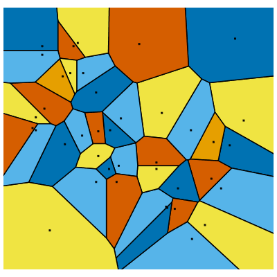
The VoronoiDiagram command computes and plots the Voronoi diagram of a set of input points. 

 

 

 

 

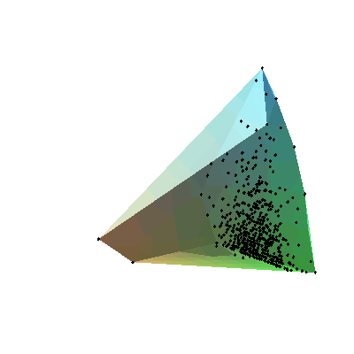
The ConvexHull command can also compute with sets of points in higher dimensions. Here we pick some random points in 3-D, where the x-coordinates, y-coordinates, and z-coordinates are chosen according to different probability distributions: the x-coordinates are the absolute values of samples from Student's t-distribution; the y-coordinates are sampled from a standard normal distribution; and the z-coordinates come from a geometric distribution. 

 

 

 

 

 

 

 

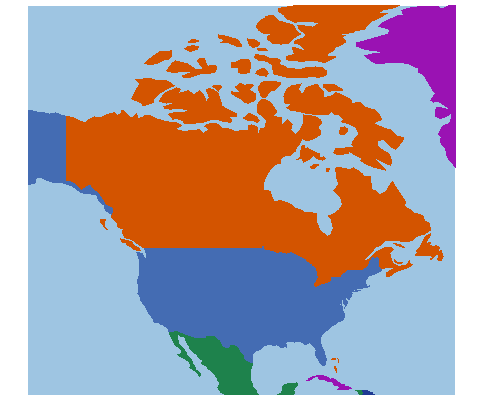
The following example uses polygon data from a section of the built-in world map. This finds all land areas that intersect with the given viewport. 

 

 

 

 

 

 

 

 

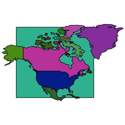
There are 41 polygons representing various elements of this map. Such polygons will be displayed throughout this example, using the procedure in the Code Edit Region below, along with additional code to help with colors. 

 

 

 

 

Remove the polygon representing the background (and the oceans). 

 

 

 

In this example, every other polygon has more than four vertices, so that is an easy criterion. 

 

 

 

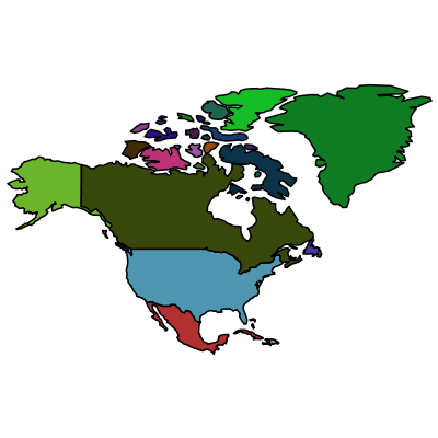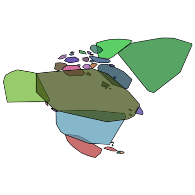
This first demonstration uses the ConvexHull command. 

 

 

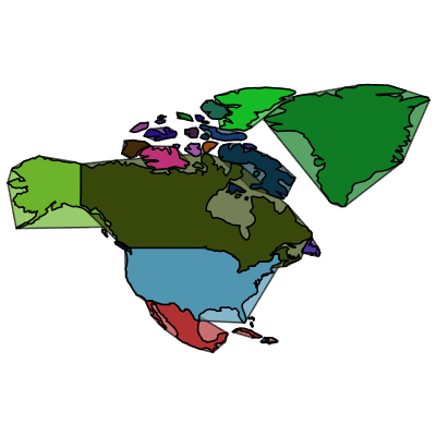
It returns the indices of the points occurring in a convex hull. You can easily show these convex hulls as follows: 

 

 

 

 

 

For the rest of this document, you will work with a single polygon. Use the one for which the area of the convex hull is largest: 

 

 

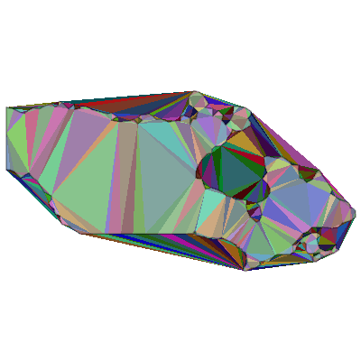
The DelaunayTriangulation of a set of points subdivides the convex hull of these points into triangles in a way that avoids long and thin triangles as much as possible. 

 

 

 

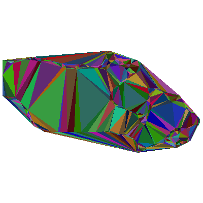This overlay shows that some of the triangles fall inside the given polygon, and some fall outside. This is because the input is interpreted as a point cloud, not an ordered polygon. 

 

 

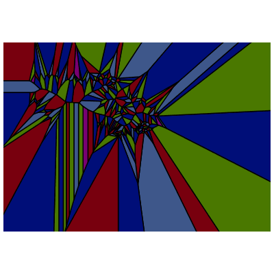
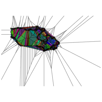
A VoronoiDiagram is a diagram that shows the dual of a Delaunay triangulation. 

 

 

 

 

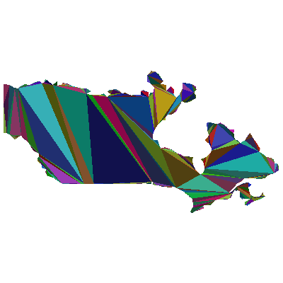
The PolygonTriangulation command interprets its argument as a polygon, that is, an ordered sequence of points, in contrast with the other commands mentioned so far, which each interprets its argument as an unordered set of points. It subdivides this polygon into triangles, trying to avoid triangles that are long and narrow.