
Maple provides numerous connectivity options with other software tools, from data import and export using a wide variety of formats, to code generation, external calling, internet connectivity, and much more. Maple 2018 expands and enhances Maple’s connectivity toolset in several ways.
Maple 2018 is now packaged with a Python 3.6 kernel.
The Python kernel is linked to Maple. This means you can execute Python scripts, and return results to Maple.
Everyone who installs Maple will also have access to a Python interpreter with a selection of useful Python libraries. In Maple, with(Python); loads a small set of tools to help execute commands, inspect variables, and interact with Python.
![]()
Arbitrary strings can be parsed and evaluated:
![]()
![]()
![]()
![]()
Here's a slightly longer string to parse and evaluate after importing the "statistics" package:
![]()
![]()
Evaluating as a string is easy and flexible, but you can go even further and make Python functions look like native Maple functions:
![]()
![]()
![]()
![]()
![]()
![]()
 |
Module :- member notation can be used to class methods:
![]()
![]()
![]()
![]()
Here is a more involved example that uses a Python package for HTML parsing and manipulation.
![]()
![]()
![]()
![]()
![]()
![]()
![]()
![]()
New procedures can be defined from Maple:
![]()
![]()
![]()
Options are available to control how results come back to Maple. Above we see 'output'='none' to prevent any result from coming back. Next, we'll use 'output' = 'python' to avoid converting back to a Maple object; and instead capture an object reference, in this case to an empty string. This allows us access to Python string methods in the result.
![]()
![]()
The Python process is in a separate memory space than Maple, and can be stopped and restarted at any time.
![]()
![]()
![]()
![]()
| Error, (in Python:-GetVariable) name 'a' is not defined |
![]()
Maple 2018 includes a new package, DeepLearning, which offers an API to a subset of the TensorFlow toolset for machine learning using neural networks.
Here we perform least-squares regression to fit a Fourier series to a set of sample data given by:
![]()
![Points := rtable(1 .. 8, 1 .. 2, [[0., 2.1], [1., -1.5], [2., -3.1], [3., 6.3], [4., 8.2], [5., 11.5], [6., 12.7], [7., 8.4]], subtype = Matrix); -1](Connectivity/Connectivity_61.gif)
The general formula for a Fourier series with ![]() terms and coefficients
terms and coefficients ![]() is given by:
is given by:
![]()
For this example we take ![]() :
:![]()
We first declare a sequence of variables in the deep learning graph corresponding to each ![]() and
and ![]() :
:
![]()
![]()
![]()
![]()
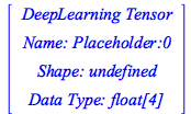
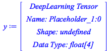
We can now define placeholders to hold the sample x- and y-values against which we want to fit ![]() :
:
![]()
 |
![]()
 |
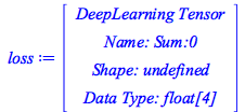
We can now define a least-squares distance function which we aim to minimize:
![]()
 |
![]()
![]()
 |
With the structure of our deep learning graph defined, we can proceed to train it on sample data. After initializing the session, we run 1000 training cycles using the training data.
![]()
![]()
![]()
![]()
![]()
![]()
We can now query the state of the trained model for the present value of the loss function:
![]()
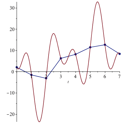
As this is a small value, we have a close fit for the data. We can then obtain the final value of the parameters from the trained model.
![]()
 |
![]()
 |
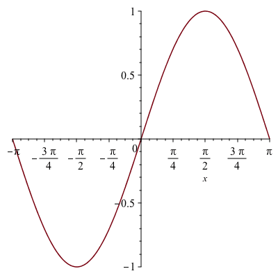
Finally, we can visualize the result:
![]()
![]()
 |
Here we use a deep neural network to classify the famous Iris flower data set collected by Edgar Anderson and made famous by Ronald Fisher. This data set includes 150 distinct observations of iris flowers, each of which consists of four empirical observations (sepal length, sepal width, petal length, and petal width) along with a classification into one of three known species (I. setosa, I. versicolor, and I. virginica).
We will repeat here the classical task for which this data set is used: attempting prediction of the species based on the four measured quantities
Training and Test Data
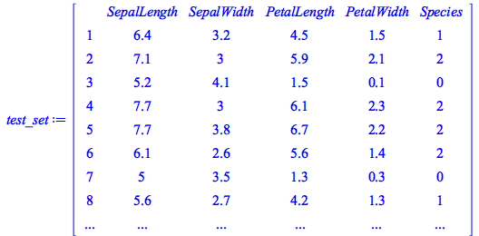
We have divided the data in into training and test data: the former is used to build the model, the latter is used to test its predictive accuracy.
![]()
![DataFrame(_rtable[18446744074844130830], rows = [1, 2, 3, 4, 5, 6, 7, 8, 9, 10, 11, 12, 13, 14, 15, 16, 17, 18, 19, 20, 21, 22, 23, 24, 25, 26, 27, 28, 29, 30, 31, 32, 33, 34, 35, 36, 37, 38, 39, 40, ...](Connectivity/Connectivity_105.gif) |
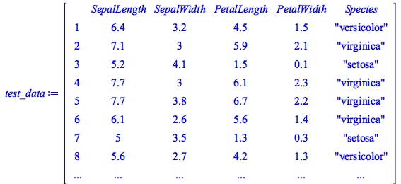 |
We see that this data set has 150 samples (120 for training and 30 for testing) and that the Species column has three distinct species:![]()
![]()
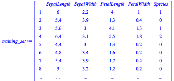
To simplify things we will replace the strings designating the species classification with the numbers 0,1,2 (corresponding to setosa, versicolor, and virginica, respectively):
![]()
 |
![]()
 |
Training the Deep Neural Network Model
With our data prepared, we can now actually define and train the model.
![]()
Our first step is to define a feature for each of the four observed quantities in the test data minus the final one (species) which we aim to predict:
![]()
![]()
We can now define a deep neural network classifier with these features. It has 3 classes because there are 3 species of iris in the dataset.
![]()
| WARNING:tensorflow:Using temporary folder as model directory: C:\Users\sforrest\AppData\Local\Temp\tmpl9jkz4pj |
We are now ready to train the model.
![]()
 |
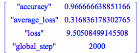
Now trained, we can evaluate the classifier on the test set, and we see that we have achieved 96.7% predictive accuracy:
![]()
 |
We can now build a predictor function that takes an arbitrary set of measurements as a DataSeries and returns a prediction:
![]()
Using a Trained Model
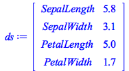
With this we can take an arbitrary new point, and generate a prediction from the trained model:
![]()
 |
![]()
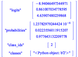 |
The probabilities field in the above result records the estimated probabilities for each class.
In this case, the model estimates a 97.8% probability that this particular sample is class 2, and therefore predicts that it is I. virginica.
The CanonicalPath command resolves any relative directories and symbolic links present in a given file path to construct a canonical version of this path.
| > |
| > |
The IsLink command tests whether a given file path corresponds to a symbolic link.
| > |
ToRecord formats an XML tree as a nested record
| > |
This example shows how repeated elements are put into a list, and the order they occurred can be deduced from the _order export.
| > |
| > |
| > |
|
<doc> <a>1</a> <b>2</b> <a>3</a></doc> |
| > |
| > |
| > |
| > |
The new MapleTA:-QTI command converts IMS Question & Test Interoperability (QTI) files into Maple T.A./Möbius course module.
OpenMaple enhances Java connectivity with several new commands, including toBigDecimal, toBigInteger, Relation, evalBoolean, lhs and set.