New Features in Maple 2018 - Partial Differential Equations - Maplesoft

What's New in Maple 2018

Partial Differential Equations


For Partial differential equations with boundary condition (PDE and BC), problems in three independent variables can now be solved, and more problems in two independent variables are now solved.  


PDE&BC problems in three independent variables for bounded spatial domains can now be solved

We are now able to solve 3-variable PDE&BC problems in bounded spatial domains through separation of variables by product and eigenfunction expansion. The example problems and corresponding descriptions below are taken from: Articolo, George A. Partial Differential Equations and Boundary Value Problems with Maple. 2nd ed., Elsevier Academic Press, 2009.


A homogeneous diffusion PDE in two bounded spatial dimensions

The temperature distribution in thin plates whose lateral surfaces are insulated, in the bounded domain is sought. The problem is represented as follows (Articolo, p.396): 

> pde[1] := diff(u(x, y, t), t) = `+`(`*`(`/`(1, 10), `*`(diff(u(x, y, t), x, x))), `*`(`/`(1, 10), `*`(diff(u(x, y, t), y, y)))); -1

with the boundary and initial conditions: 

> iv[1] := u(0, y, t) = 0, u(1, y, t) = 0, u(x, 0, t) = 0, u(x, 1, t) = 0, u(x, y, 0) = `*`(x, `*`(`+`(1, `-`(x)), `*`(`+`(1, `-`(y)), `*`(y)))); -1

> pdsolve([pde[1], iv[1]], u(x, y, t))

u(x, y, t) = Sum(Sum(`+`(`-`(`/`(`*`(16, `*`(`+`(`-`(`^`(-1, `+`(n1, n))), `^`(-1, n1), `^`(-1, n), `-`(1)), `*`(sin(`*`(n, `*`(Pi, `*`(x)))), `*`(sin(`*`(n1, `*`(Pi, `*`(y)))), `*`(exp(`+`(`-`(`*`(`/...

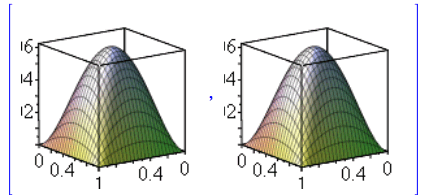
One way to verify that this solution satisfies the initial condition is to plot u(x, y, 0) = `*`(x, `*`(`+`(1, `-`(x)), `*`(`+`(1, `-`(y)), `*`(y)))) together with its series representation (below we use the first 10000 terms in the solution) in the corresponding range, in this case x = 0 .. 1, y = 0 .. 1. 

> map(plot3d, [subs(t = 0, infinity = 100, rhs(u(x, y, t) = Sum(Sum(`+`(`-`(`/`(`*`(16, `*`(`+`(`-`(`^`(-1, `+`(n1, n))), `^`(-1, n1), `^`(-1, n), `-`(1)), `*`(sin(`*`(n, `*`(Pi, `*`(x)))), `*`(sin(`*`(...

[INTERFACE_PLOT3D(GRID(0. .. 1., 0. .. 1., Array(1..49, 1..49, {(1, 1) = .0, (1, 2) = .0, (1, 3) = .0, (1, 4) = .0, (1, 5) = .0, (1, 6) = .0, (1, 7) = .0, (1, 8) = .0, (1, 9) = .0, (1, 10) = .0, (1, 1...

A homogeneous diffusion PDE with heat loss in two bounded spatial dimensions

The temperature distribution in thin plates whose lateral surfaces are experiencing heat loss proportional to the plate and surrounding temperatures in a bounded domain is sought. The problem is represented as follows (Articolo, p. 401): 

> pde[2] := diff(u(x, y, t), t) = `+`(`*`(`/`(1, 10), `*`(diff(u(x, y, t), x, x))), `*`(`/`(1, 10), `*`(diff(u(x, y, t), y, y))), `-`(`*`(`/`(1, 5), `*`(u(x, y, t))))); -1

with the boundary and initial conditions: 

> iv[2] := (D[1](u))(0, y, t) = 0, u(1, y, t) = 0, u(x, 0, t) = 0, (D[2](u))(x, 1, t) = 0, u(x, y, 0) = `*`(`+`(`-`(`*`(`^`(x, 2))), 1), `*`(`+`(1, `-`(`*`(`/`(1, 2), `*`(y)))), `*`(y))); -1

> pdsolve([pde[2], iv[2]], u(x, y, t))

u(x, y, t) = Sum(Sum(`+`(`/`(`*`(512, `*`(`^`(-1, n), `*`(cos(`+`(`*`(`/`(1, 2), `*`(`+`(1, `*`(2, `*`(n))), `*`(Pi, `*`(x)))))), `*`(sin(`+`(`*`(`/`(1, 2), `*`(`+`(1, `*`(2, `*`(n1))), `*`(Pi, `*`(y)...

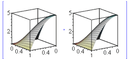
To verify that this solution satisfies the initial condition, we plot u(x, y, 0) = `*`(`+`(`-`(`*`(`^`(x, 2))), 1), `*`(`+`(1, `-`(`*`(`/`(1, 2), `*`(y)))), `*`(y))) and its series representation in the domain, which in this case is again x = 0 .. 1, y = 0 .. 1

> map(plot3d, [subs(t = 0, infinity = 100, rhs(u(x, y, t) = Sum(Sum(`+`(`/`(`*`(512, `*`(`^`(-1, n), `*`(cos(`+`(`*`(`/`(1, 2), `*`(`+`(1, `*`(2, `*`(n))), `*`(Pi, `*`(x)))))), `*`(sin(`+`(`*`(`/`(1, 2)...

[INTERFACE_PLOT3D(GRID(0. .. 1., 0. .. 1., Array(1..49, 1..49, {(1, 1) = .0, (1, 2) = 0.20615474597998933e-1, (1, 3) = 0.40798196725302105e-1, (1, 4) = 0.6054666821553681e-1, (1, 5) = 0.79861029636343...

A homogeneous wave PDE in two bounded spatial dimensions

The wave amplitude for the transverse wave propagation on a thin rectangular membrane in a medium with no damping over a finite domain is sought. The problem is represented as follows (Articolo, p. 425): 

> pde[3] := diff(u(x, y, t), t, t) = `+`(`*`(`/`(1, 4), `*`(diff(u(x, y, t), x, x))), `*`(`/`(1, 4), `*`(diff(u(x, y, t), y, y)))); -1

with the boundaries x = 0, x = Pi unsecured, boundaries y = 0, y = Pi secured, and initial conditions as follows: 

> iv[3] := (D[1](u))(0, y, t) = 0, (D[1](u))(Pi, y, t) = 0, u(x, 0, t) = 0, u(x, Pi, t) = 0, (D[3](u))(x, y, 0) = 0, u(x, y, 0) = `*`(x, `*`(y, `*`(`+`(Pi, `-`(y))))); -1

> pdsolve([pde[3], iv[3]], u(x, y, t))

u(x, y, t) = `+`(Sum(`+`(`-`(`/`(`*`(2, `*`(`+`(`^`(-1, n), `-`(1)), `*`(sin(`*`(n, `*`(y))), `*`(cos(`+`(`*`(`/`(1, 2), `*`(n, `*`(t))))))))), `*`(`^`(n, 3))))), n = 1 .. infinity), Sum(Sum(`+`(`/`(`...

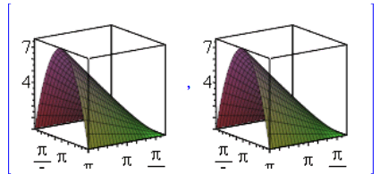
We verify the initial condition by comparing plots of both the initial condition function u(x, y, 0) = `*`(x, `*`(y, `*`(`+`(Pi, `-`(y))))) and its series representation: 

> map(plot3d, [subs(t = 0, infinity = 100, rhs(u(x, y, t) = `+`(Sum(`+`(`-`(`/`(`*`(2, `*`(`+`(`^`(-1, n), `-`(1)), `*`(sin(`*`(n, `*`(y))), `*`(cos(`+`(`*`(`/`(1, 2), `*`(n, `*`(t))))))))), `*`(`^`(n, ...

[INTERFACE_PLOT3D(GRID(0. .. 3.14159265358979, 0. .. 3.14159265358979, Array(1..49, 1..49, {(1, 1) = .0, (1, 2) = 0.1281574751933967e-2, (1, 3) = 0.2508770252619752e-2, (1, 4) = 0.3681398436884642e-2,...

A homogeneous wave PDE (with damping) in two bounded spatial dimensions  

The wave amplitude for the transverse wave propagation on a thin rectangular membrane in a medium with damping over a finite domain is sought. The problem is represented as follows (Articolo, p. 468): 

> pde[4] := diff(u(x, y, t), t, t) = `+`(`*`(`/`(1, 4), `*`(diff(u(x, y, t), x, x))), `*`(`/`(1, 4), `*`(diff(u(x, y, t), y, y))), `-`(`*`(`/`(1, 10), `*`(diff(u(x, y, t), t))))); -1

with the boundaries x = 0, y = 0 held secure, boundaries x = 1, y = 1 unsecure, and initial conditions as follows: 

> iv[4] := u(0, y, t) = 0, (D[1](u))(1, y, t) = 0, u(x, 0, t) = 0, (D[2](u))(x, 1, t) = 0, u(x, y, 0) = 0, (D[3](u))(x, y, 0) = `*`(x, `*`(`+`(1, `-`(`*`(`/`(1, 2), `*`(x)))), `*`(`+`(1, `-`(`*`(`/`(1, ...

> pdsolve([pde[4], iv[4]], u(x, y, t))

u(x, y, t) = Sum(Sum(`+`(`/`(`*`(5120, `*`(sin(`+`(`*`(`/`(1, 2), `*`(`+`(1, `*`(2, `*`(n))), `*`(Pi, `*`(x)))))), `*`(sin(`+`(`*`(`/`(1, 2), `*`(`+`(1, `*`(2, `*`(n1))), `*`(Pi, `*`(y)))))), `*`(exp(...

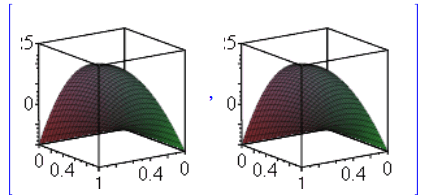
To verify the initial condition, we compare the plots of both the initial condition function (D[3](u))(x, y, 0) = `*`(x, `*`(`+`(1, `-`(`*`(`/`(1, 2), `*`(x)))), `*`(`+`(1, `-`(`*`(`/`(1, 2), `*`(y)))), `*`(y)))) and its series representation: 

> map(plot3d, [subs(t = 0, infinity = 100, diff(rhs(u(x, y, t) = Sum(Sum(`+`(`/`(`*`(5120, `*`(sin(`+`(`*`(`/`(1, 2), `*`(`+`(1, `*`(2, `*`(n))), `*`(Pi, `*`(x)))))), `*`(sin(`+`(`*`(`/`(1, 2), `*`(`+`(...

[INTERFACE_PLOT3D(GRID(0. .. 1., 0. .. 1., Array(1..49, 1..49, {(1, 1) = .0, (1, 2) = .0, (1, 3) = .0, (1, 4) = .0, (1, 5) = .0, (1, 6) = .0, (1, 7) = .0, (1, 8) = .0, (1, 9) = .0, (1, 10) = .0, (1, 1...

More PDE&BC problems in two independent variables for bounded spatial domains can be solved

The code for solving PDE&BC problems in bounded spatial domains through separation by product and eigenfunction expansion continues to grow.  


Solving more problems with periodic boundary conditions

A problem involving the diffusion PDE: 

> pde[5] := diff(u(x, t), t) = `*`(k, `*`(diff(u(x, t), x, x))); -1

> iv[5] := u(x, 0) = f(x), u(`+`(`-`(l)), t) = u(l, t), (D[1](u))(`+`(`-`(l)), t) = (D[1](u))(l, t); -1

> `assuming`([pdsolve([pde[5], iv[5]], u(x, t))], [`<`(0, l)])

Typesetting:-mprintslash([u(x, t) = `+`(`/`(`*`(`/`(1, 2), `*`(`+`(`*`(2, `*`(Sum(`/`(`*`(`+`(`*`(Int(`*`(f(x), `*`(sin(`/`(`*`(n, `*`(Pi, `*`(x))), `*`(l))))), x = `+`(`-`(l)) .. l), `*`(sin(`/`(`*`(...

A problem involving the Laplace PDE in cylindrical coordinates: 

> pde[6] := `+`(`/`(`*`(diff(`*`(r, `*`(diff(u(r, theta), r))), r)), `*`(r)), `/`(`*`(diff(u(r, theta), theta, theta)), `*`(`^`(r, 2)))) = 0; -1

> iv[6] := u(a, theta) = f(theta), u(r, `+`(`-`(Pi))) = u(r, Pi), (D[2](u))(r, `+`(`-`(Pi))) = (D[2](u))(r, Pi); -1

> `assuming`([pdsolve([pde[6], iv[6]], u(r, theta), HINT = boundedseries)], [`<`(0, a)])

Typesetting:-mprintslash([u(r, theta) = `+`(`/`(`*`(`/`(1, 2), `*`(`+`(`*`(2, `*`(Sum(`/`(`*`(`^`(r, n), `*`(`+`(`*`(Int(`*`(f(theta), `*`(sin(`*`(n, `*`(theta))))), theta = `+`(`-`(Pi)) .. Pi), `*`(s...

Another problem involving the heat PDE: 

> pde[7] := diff(u(x, t), t) = diff(u(x, t), x, x); -1

> iv[7] := u(x, 0) = f(x), u(-1, t) = 0, u(1, t) = 0; -1

> pdsolve([pde[7], iv[7]], u(x, t))

Typesetting:-mprintslash([u(x, t) = Sum(`*`(`+`(`*`(Int(`*`(f(x), `*`(sin(`*`(n, `*`(Pi, `*`(x)))))), x = -1 .. 1), `*`(sin(`*`(n, `*`(Pi, `*`(x)))), `*`(exp(`+`(`*`(`/`(1, 4), `*`(t, `*`(`^`(Pi, 2), ...

Solving more problems with non-homogeneous boundary conditions 

A problem involving the heat PDE:  

> pde[8] := diff(u(x, t), t) = diff(u(x, t), x, x); -1

> iv[8] := u(0, t) = 20, u(1, t) = 50, u(x, 0) = 0; -1

> pdsolve([pde[8], iv[8]], u(x, t))

u(x, t) = `+`(20, `*`(30, `*`(x)), Sum(`/`(`*`(`+`(`-`(40), `*`(100, `*`(`^`(-1, n)))), `*`(sin(`*`(n, `*`(Pi, `*`(x)))), `*`(exp(`+`(`-`(`*`(t, `*`(`^`(Pi, 2), `*`(`^`(n, 2)))))))))), `*`(n, `*`(Pi))...

A problem involving the heat PDE with a source: 

> pde[9] := `+`(diff(u(x, t), t), `*`(k, `*`(diff(u(x, t), x, x))), k); -1

> iv[9] := u(x, 0) = f(x), u(0, t) = A, u(L, t) = B; -1

> pdsolve([pde[9], iv[9]], u(x, t))

Typesetting:-mprintslash([u(x, t) = `+`(`/`(`*`(`/`(1, 2), `*`(`+`(`*`(2, `*`(Sum(`+`(`-`(`/`(`*`(Int(`+`(`*`(2, `*`(`+`(`-`(`*`(f(x), `*`(L))), `*`(`/`(1, 2), `*`(`^`(L, 2), `*`(x))), `*`(`+`(`-`(`*`...

Solving more problems with a source term in the PDE 

A diffusion problem with a source function f(x, t)

> pde[10] := diff(u(x, t), t) = `+`(`*`(k, `*`(diff(u(x, t), x, x))), f(x, t)); -1

> iv[10] := u(0, t) = 0, u(l, t) = 0, u(x, 0) = g(x); -1

> `assuming`([pdsolve([pde[10], iv[10]], u(x, t))], [`and`(`<=`(0, x), `<=`(x, l))]); 1

Typesetting:-mprintslash([u(x, t) = `+`(Sum(`+`(`/`(`*`(2, `*`(Int(`*`(g(x), `*`(sin(`/`(`*`(n1, `*`(Pi, `*`(x))), `*`(l))))), x = 0 .. l), `*`(sin(`/`(`*`(n1, `*`(Pi, `*`(x))), `*`(l))), `*`(exp(`+`(...

Improvements to the ability to solve problems with the Laplace PDE

In cylindrical coordinates:  

> pde[11] := `+`(`/`(`*`(`+`(diff(u(r, theta), r), `*`(r, `*`(diff(u(r, theta), r, r))))), `*`(r)), `/`(`*`(diff(u(r, theta), theta, theta)), `*`(`^`(r, 2)))) = 0; -1

> iv[11] := u(0, theta) = 0, u(1, theta) = `*`(theta, `*`(`+`(`*`(`/`(1, 3), `*`(Pi)), `-`(theta)))), u(r, 0) = 0, u(r, `+`(`*`(`/`(1, 3), `*`(Pi)))) = 0; -1

> `assuming`([pdsolve([pde[11], iv[11]], u(r, theta))], [`<`(0, r), `and`(`<`(0, theta), `<`(theta, `+`(`*`(`/`(1, 3), `*`(Pi)))))])

u(r, theta) = Sum(`/`(`*`(`+`(`*`(`+`(`-`(`*`(_C5(n), `*`(Pi, `*`(`^`(n, 3))))), `-`(`*`(`/`(4, 9), `*`(`^`(-1, n)))), `/`(4, 9)), `*`(`^`(r, `+`(`*`(3, `*`(n)))))), `*`(_C5(n), `*`(`^`(r, `+`(`-`(`*`...

Improvements to the solving of problems for which a bounded solution is sought

Solutions for this Laplace PDE problem are shown for the general problem, and then for the bounded problem (with

> pde[12] := `+`(`/`(`*`(diff(u(r, theta), r)), `*`(r)), diff(u(r, theta), r, r), `/`(`*`(diff(u(r, theta), theta, theta)), `*`(`^`(r, 2)))) = 0; -1

> iv[12] := u(1, theta) = f(theta), u(r, 0) = 0, u(r, `+`(`*`(`/`(1, 3), `*`(Pi)))) = 0; -1

> `assuming`([pdsolve([pde[12], iv[12]])], [`and`(`<`(0, r), `<=`(r, 1)), `and`(`<`(0, theta), `<=`(theta, `+`(`*`(`/`(1, 3), `*`(Pi)))))])

Typesetting:-mprintslash([u(r, theta) = Sum(`/`(`*`(sin(`+`(`*`(3, `*`(n, `*`(theta))))), `*`(`+`(`*`(6, `*`(`^`(r, `+`(`*`(3, `*`(n)))), `*`(Int(`*`(f(theta), `*`(sin(`+`(`*`(3, `*`(n, `*`(theta)))))...

> `assuming`([pdsolve([pde[12], iv[12]], HINT = boundedseries)], [`and`(`<`(0, r), `<=`(r, 1)), `and`(`<`(0, theta), `<=`(theta, `+`(`*`(`/`(1, 3), `*`(Pi)))))])

Typesetting:-mprintslash([u(r, theta) = Sum(`+`(`/`(`*`(6, `*`(Int(`*`(f(theta), `*`(sin(`+`(`*`(3, `*`(n, `*`(theta))))))), theta = 0 .. `+`(`*`(`/`(1, 3), `*`(Pi)))), `*`(`^`(r, `+`(`*`(3, `*`(n))))...

Another problem with a Laplace PDE for which a bounded solution is sought: 

> pde[13] := `+`(`/`(`*`(`+`(diff(u(r, theta), r), `*`(r, `*`(diff(u(r, theta), r, r))))), `*`(r)), `/`(`*`(diff(u(r, theta), theta, theta)), `*`(`^`(r, 2)))) = 0; -1

> iv[13] := u(1, theta) = `*`(theta, `*`(`+`(1, `-`(`/`(`*`(`/`(3, 2), `*`(theta)), `*`(Pi)))))), u(r, 0) = 0, (D[2](u))(r, `+`(`*`(`/`(1, 3), `*`(Pi)))) = 0; -1

> pdsolve([pde[13], iv[13]], u(r, theta), HINT = boundedseries)

u(r, theta) = Sum(`+`(`/`(`*`(`/`(16, 3), `*`(`^`(r, `+`(`/`(3, 2), `*`(3, `*`(n)))), `*`(sin(`+`(`*`(3, `*`(n, `*`(theta))), `*`(`/`(3, 2), `*`(theta))))))), `*`(`^`(Pi, 2), `*`(`^`(`+`(1, `*`(2, `*`...

Solving problems for which there are both homogeneous and non-homogeneous boundary conditions for each independent variable 

In this kind of problem, we don't directly arrive at a Sturm-Liouville problem after separation of variables, but instead must solve two simplified versions of the problem and then combine those answers to solve the original problem: 


> pde[14] := `+`(diff(u(x, y), x, x), diff(u(x, y), y, y)) = 0; -1

> iv[14] := u(0, y) = `+`(`-`(`*`(`^`(y, 2))), y), (D[1](u))(1, y) = 0, u(x, 0) = 0, u(x, 1) = `*`(x, `*`(`+`(1, `-`(`*`(`/`(1, 2), `*`(x)))))); -1

> `assuming`([pdsolve([pde[14], iv[14]], u(x, y))], [`and`(`<`(0, x), `<=`(x, 1))])

u(x, y) = `+`(Sum(`+`(`-`(`/`(`*`(4, `*`(`+`(`^`(-1, n), `-`(1)), `*`(sin(`*`(Pi, `*`(y, `*`(n)))), `*`(`+`(exp(`+`(`-`(`*`(Pi, `*`(n, `*`(`+`(x, `-`(2)))))))), exp(`*`(n, `*`(Pi, `*`(x))))))))), `*`(...

General improvements

A non-linear PDE: 

> pde[15] := `+`(diff(u(x, y), x), `*`(u(x, y), `*`(diff(u(x, y), y)))) = 0; -1

> iv[15] := u(x, 0) = `/`(1, `*`(`+`(x, 1))); -1

> pdsolve([pde[15], iv[15]], u(x, y))

u(x, y) = `/`(`*`(`+`(y, 1)), `*`(`+`(x, 1)))

A wave PDE problem:

> pde[16] := `+`(`*`(100, `*`(diff(u(x, t), x, x)))) = diff(u(x, t), t, t); -1

> iv[16] := u(0, t) = 0, u(2, t) = 0, u(x, 0) = `+`(`*`(32, `*`(sin(`*`(Pi, `*`(x))))), `*`(`^`(e, 2), `*`(sin(`+`(`*`(3, `*`(Pi, `*`(x))))))), `*`(25, `*`(sin(`+`(`*`(6, `*`(Pi, `*`(x)))))))), (D[2](u)...

> `assuming`([pdsolve([pde[16], iv[16]], u(x, t))], [`and`(`<`(0, x), `<=`(x, 2))])

u(x, t) = `+`(`/`(`*`(`/`(1, 50), `*`(`+`(`*`(50, `*`(sin(`+`(`*`(3, `*`(Pi, `*`(x))))), `*`(`^`(e, 2), `*`(cos(`+`(`*`(30, `*`(Pi, `*`(t))))), `*`(Pi))))), `*`(1600, `*`(sin(`*`(Pi, `*`(x))), `*`(cos...

Another wave PDE problem: 

> pde[17] := `+`(`*`(4, `*`(diff(u(x, t), x, x)))) = diff(u(x, t), t, t); -1

> iv[17] := u(0, t) = 0, u(Pi, t) = 0, u(x, 0) = 0, (D[2](u))(x, 0) = 6; -1

> `assuming`([pdsolve([pde[17], iv[17]], u(x, t))], [`and`(`<`(0, x), `<=`(x, Pi))])

u(x, t) = Sum(`+`(`-`(`/`(`*`(6, `*`(`+`(`^`(-1, n), `-`(1)), `*`(sin(`*`(n, `*`(x))), `*`(sin(`+`(`*`(2, `*`(n, `*`(t))))))))), `*`(Pi, `*`(`^`(n, 2)))))), n = 1 .. infinity)