Computational Geometry

Maple 2019 includes a number of new commands in the ComputationalGeometry package. 

PointOrientation 

This command gives a very efficient test of the orientation of three points in two dimensions or four points in three dimensions. Either "cw" or "ccw" for points in clockwise or counterclockwise order or "degenerate" if they are colinear or coplanar. 

>	with(ComputationalGeometry):

 

>	a := [0,0]: b := [1,1]: c := [0.4,0.8]: d := [0.8,0.4]: e:=[0.5,0.5]:

 

>	PointOrientation(a, b, c);

 

 

>	PointOrientation(a, b, d);

 

 

>	PointOrientation(a, b, e);

 

 

 

The most efficient way to use this command is on a large array of point coordinates. PointOrientation works on these in place without having to copy the points into a new memory location making it efficient when doing many of these calculations at a time. 

>	A := Array( [a,b,c,d,e], datatype=float[8], order=C_order );

 

 

>	PointOrientation( A, [1,2,5]);

 

 

>	a := [0,0,0]: b := [1,1,0]: c := [0.4,0.8,0]: d := [0.8,0.4,-1]: e := [0.5,0.5,1]: f := [0.5,0.5,0]:

 

>	PointOrientation(a, b, c, d);

 

 

>	PointOrientation(a, b, c, e);

 

 

>	PointOrientation(a, b, c, f);

 

 

PointInCircle 

This command gives a very efficient test to determine if a fourth point is inside a circle defined by three points. Like PointOrientation, the PointInCircle command also has an efficient mode for arrays of points. 

 

>	a := [0,0]: b := [1,1]: c := [0,1]: d := [0.5,1.25]: e:=[0.25,0.75]: f:=[1,0]:

 

>

plots:-display(plottools:-point([a,b,c,d,e,f],symbolsize=20),              plots:-textplot([d[], "d"], align=["above", "left"]),              plots:-textplot([e[], "e"], align=["above", "left"]),              plots:-textplot([f[], "f"], align=["above", "left"]),              plottools:-circle([1/2,1/2], sqrt(2)/2, style=line), axes=box );

 

 

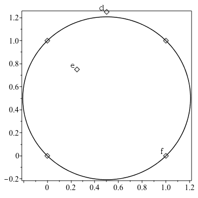>	PointInCircle(a, b, c, d);

 

 

>	PointInCircle(a, b, c, e);

 

 

>	PointInCircle(a, b, c, f);

 

 

PointOnSegment 

This command gives an accurate test to determine if a third point is on a line segment defined by two points. Like PointOrientation, the PointOnSegment command also has an efficient mode for arrays of points. 

>	a := [0,0]: b := [1,1]: c := [0.4,0.4]: d := [1.1,1.1]: e:=[0.5,0.55]:

 

>

plots:-display(plottools:-point([a,b,c,d,e],symbolsize=20),               plots:-textplot([c[], "c"], align=["above", "left"]),               plots:-textplot([d[], "d"], align=["below", "left"]),               plots:-textplot([e[], "e"], align=["above", "left"]),               plottools:-line(a, b), axes=box );

 

 

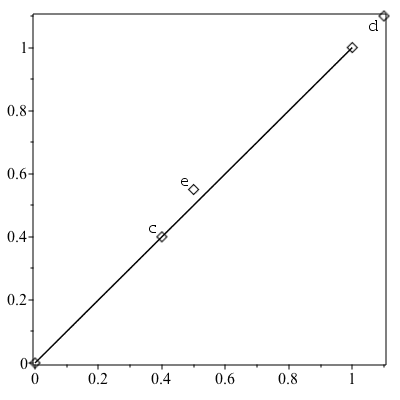>	PointOnSegment(c, [a, b]);

 

 

>	PointOnSegment(d, [a, b]);

 

 

>	PointOnSegment(e, [a, b]);

 

 

 

SegmentsIntersect 

This command gives an efficient test to determine if two line segments intersect. Like PointOrientation, the SegmentsIntersect command also has an efficient mode for arrays of points. 

>	SegmentsIntersect([[0,0], [1,1]], [[0,1], [1,0]]);

 

 

>	L := [[1,0], [1,5]]:

 

>

K := [ [[1,-2], [1,-1]], [[0,1], [0,3]], [[2,1], [2,3]], [[1,6.5], [1,8]],      [[1,6], [1.5,8]], [[0.5,4], [1.5,7]], [[0.5, 0.5], [1, -0.75]],      [[1,5], [1.5,6]], [[1,4.5], [1.5,5]], [[.5,3.75], [1.5,3.5]],      [[1,2.5], [1,3.5]], [[0.5,1.5], [1,2]], [[1,0], [1.5,-2]],      [[1, 0.5], [1, -0.5]] ]:

 

>	plots:-display( plottools:-line(L[], legend="L", color="Dalton 2", thickness=3), seq(plottools:-line(K[i][], legend="K " || i, color="Blue"), i=1..7), seq(plottools:-line(K[i][], legend="K " || i, color="Green"), i=8..14), axes=boxed, style=pointline);

 

 

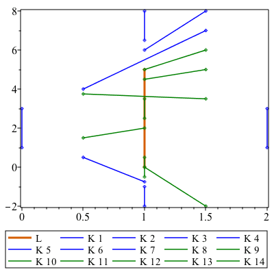None of the blue segments intersect L (orange). 

>	{ seq(SegmentsIntersect(L, K[i]), i=1..7) };

 

 

All of the green segments intersect L. 

>	{ seq(SegmentsIntersect(L, K[i]), i=8..14) };

 

 

 

MultiSegmentIntersect 

The MultiSegmentIntersect command uses a sweep line algorithm to determine if the collections of line segments have intersections. It can be used, to name a few cases, to test if a line segment intersects a polygon, test if a collection of segments has any intersections, or find all the intersections in a collection of polygons. 

 

Here L is a collection of line segments, and M is a list of the vertices of a polygon. 

>	L := [ [[-.5, -1], [-.5,2]], [[.5,-1], [.5,2]], [[1.5,-1], [1.5,2]], [[0.75,1.5], [1.25,0.5]], [[-.25,0], [1.25, 0]], [[.2,1], [.4,1]], [[-.25,.5], [.25,.25]], [[0, 0.5], [0, 1.5]] ]: M := [[0,0], [0,1], [1,1], [1,0]]:

 

>	plots:-display( seq(plottools:-line(L[i][], legend="L "||i, color="Red",style=pointline),i=1..nops(L)), plottools:-polygon(M,style=pointline, legend="M"), axes=none);

 

 

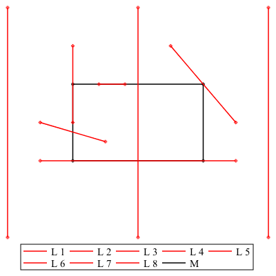>	MultiSegmentIntersect( [L[1],  M ], mode="polygon", output="truefalse" )

 

 

The fourth segment in L intersects M just once. 

>	MultiSegmentIntersect( [L[4],  M ], mode="polygon" )

 

 

The second segment in L intersects M twice, but we can use the 'lazy' option to find just one of them. 

>	MultiSegmentIntersect( [L[2],  M ], mode="polygon", lazy )

 

 

We can also find all the intersections of L and M at once by flattening L into a list of points to be treated as point pairs. 

>	MultiSegmentIntersect( [map(op,L),  M ], mode=["pairs","polygon"] )

 

 

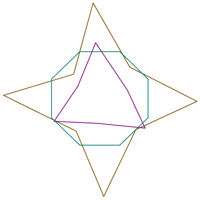
P, Q, and R are the vertices of three irregular polygons. 

>	P := op(1,plottools:-polygonbyname("8gon", inbox=[1.2,1.2])): Q := op(1,plottools:-polygonbyname("3gon", irregular, star, radius=1/2)): R := op(1,plottools:-polygonbyname("4gon", irregular, star=3, radius=3/4)):

 

 

>	theplot := plots:-display(    plottools:-polygon(P, style=line, color="Niagara 6"),    plottools:-polygon(Q, style=line, color="Niagara 5"),    plottools:-polygon(R, style=line, color="Niagara 9" ), axes=none );

 

 

 

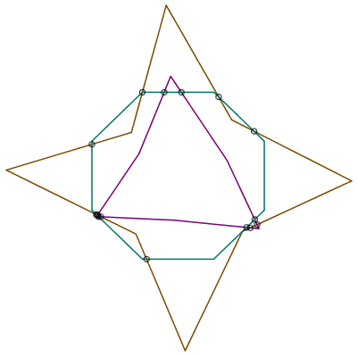
>	segints := MultiSegmentIntersect( [ P, Q, R], mode="polygon" );

 

 

 

>	plots:-display( theplot, plottools:-point( segints,               symbol="circle", 'symbolsize'=15, 'color'="Black"), axes=none );

 

 

 

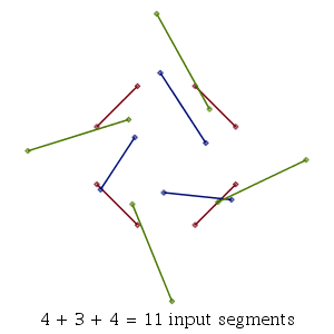
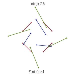
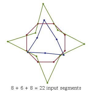
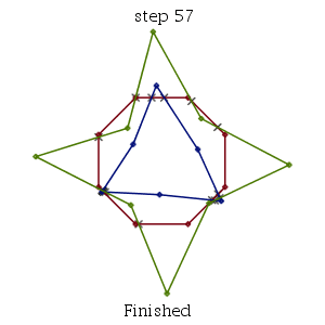
As with several other new ComputationalGeometry commands setting the infolevel of CompGeomPlot to 1 or greater will give some graphical representation of the steps of the algorithm.  In this example, we use the default mode="pairs" mode which treats the collections of points as unconnected line segments.  An infolevel value of 1 plots the input and, at the end, the intersections found.  Values of 2 or 4 will show the steps of the algorithm as it runs. 

>	infolevel[CompGeomPlot] := 1: MultiSegmentIntersect( [ P, Q, R] );

 

 

 

 

 

MultiSegmentIntersect:

MultiSegmentIntersect:

 

The mode option of MultiSegmentIntersect is meant to allow for convenience.  The command can also take a single rtable of point coordinates together with a list of lists of index pairs specifying line segment endpoints in the point rtable. 

>	M := Matrix([[P],[Q],[R]]): S := [ [seq([i,i+1], i=1..8-1), [8,1]],       [seq([8+i,8+i+1], i=1..6-1), [8+6,8+1]],       [seq([14+i,14+i+1], i=1..8-1), [14+8,14+1]] ]; infolevel[CompGeomPlot] := 1: MultiSegmentIntersect(M, S); infolevel[CompGeomPlot] := 0:

 

 

 

 

 

 

MultiSegmentIntersect:

MultiSegmentIntersect:

 

ClosestPointPair 

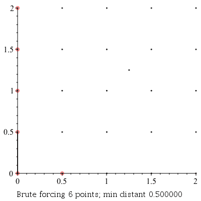
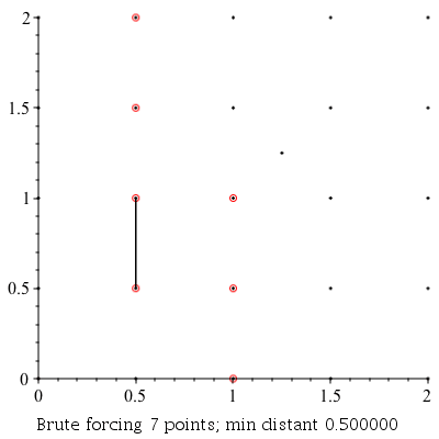
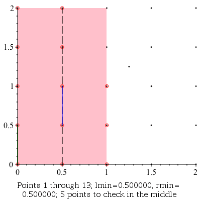
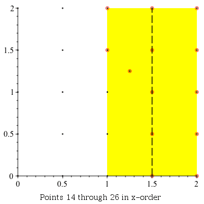
Use the ClosestPointPair command to find a closest pair of points in a collection of points in any dimension. It uses a classic divide and conquer approach. 

>	ClosestPointPair( [[0,1], [2,2], [1,1], [4,4]] );

 

 

Verbose Demonstration 

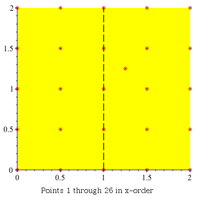
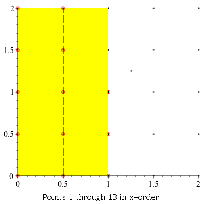
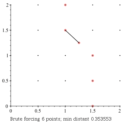
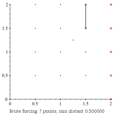
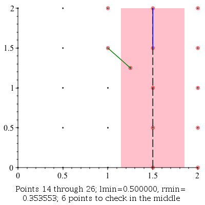
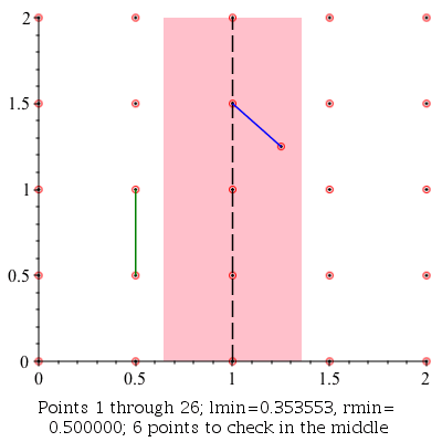
This command can be used to demonstrate the algorithm visually by setting the infolevel of CompGeomPlot to 4. 

>	infolevel[CompGeomPlot]:=4: ClosestPointPair( [seq(seq(seq([i, j], i = 0 .. 2, .5), j = 0 .. 2, .5)), [1.25, 1.25]] ); infolevel[CompGeomPlot]:=1:

ClosestPointPair:

ClosestPointPair:

ClosestPointPair:

ClosestPointPair:

ClosestPointPair:

ClosestPointPair:

ClosestPointPair:

ClosestPointPair:

ClosestPointPair:

ClosestPointPair:

Here is a slightly larger example in three dimensions. 

>	L := [seq(seq(seq([i, j, k], i = 0 .. 4, .25), j = 0 .. 4, .25), k = 0 .. 4, .25), [1.85, 1.85, 1.85]]: numelems(L);

 

 

>	(d,p) := ClosestPointPair( L ); L[p[1]],L[p[2]];

 

 

 

 

DelaunayTriangulation 

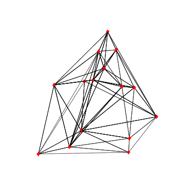
The DelaunayTriangulation command introduced in Maple 2018 now supports computing triangularizations in dimensions up to 10. 

>	m := RandomTools:-Generate(list(list(float(range=-95..95),3),15));

 

 

>	t := DelaunayTriangulation(m);

 

 

We can collect the outputs to form the polygon faces of the tetrahedrons in t and plot them. 

>	tetrahedron := A->plottools:-polygon([[A[1], A[2], A[3]], [A[1], A[2], A[4]], [A[1], A[3], A[4]], [A[2], A[3], A[4]]], style=line, color="Black"): plots:-display(   plottools:-point(m, symbolsize=20, color="Red"),   map(x->tetrahedron(m[x]),t),axes=none);

 

 

Back to What's New Overview