
Frequency Spectrum of Irregularly Sampled Data
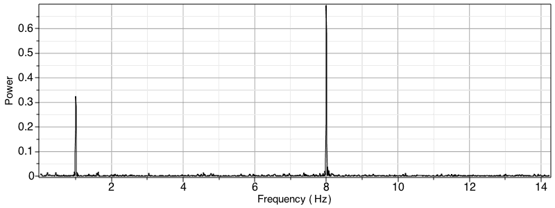
The new LSPeriodogram command uses the Lomb-Scargle technique to generate a periodogram of data sampled at irregular time intervals. This is in contrast to the standard Fourier approach (such as that used in Periodogram) which requires regularly sampled data.
| > |
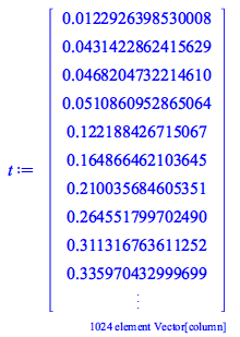
Generate an irregularly spaced vector of times
| > |
 |
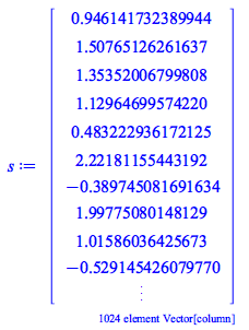
Generate a signal using frequencies of 1 Hz and 8 Hz
| > |
| > |
 |
Generate a periodogram assuming that the signal is sampled at each point in the irregularly spaced time vector
| > |
 |
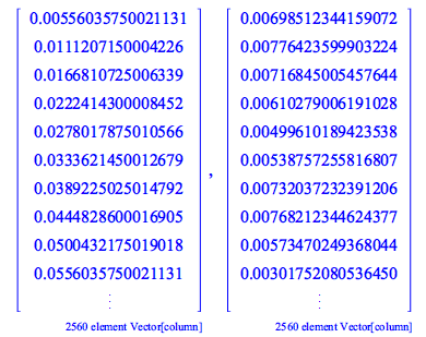
Several options allow you to specify the frequencies over which the periodogram is generated, the normalization and more. Additionally, you can also generate the numerical data used to create this plot with the LSSpectrum command.
| > |
 |
FindPeakPoints
The new FindPeakPoints command finds the peaks and valleys of 1D data sets. This versatile command offers several options that let you filter out peaks or valleys that are too close, what defines a peak or valley, and more.
Here, we find the fundamental frequency and harmonics of a violin note by locating the peak points of its periodogram. This speaker component is needed to play audio: ![]()
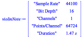
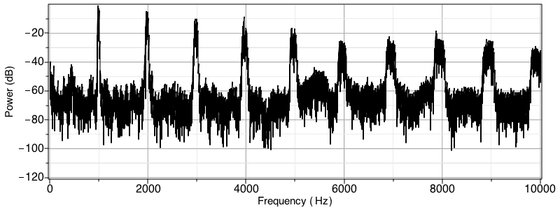
First import, play the data, and view the power spectrum.
| > |
 |
| > |
 |
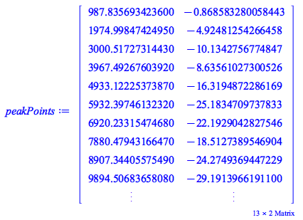
Now isolate the peak points on the periodogram, while filtering out any spurious peaks.
| > |
 |
Overlay the peak points over the periodogram
| > |
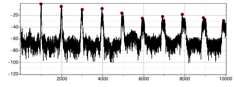 |
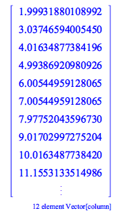
The fundamental frequency of the violin note is the first frequency in peakPoints (987.8 Hz). The other values are the harmonics (which are approximately integer multiples of the fundamental frequency)
| > |
 |
Spectrogram
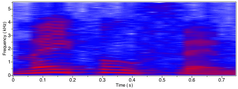
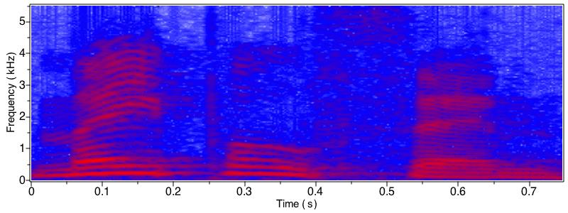
You can now specify the overlap when generating a spectrogram (in prior releases, the overlap was fixed at 50%).
Increasing overlap increases frequency resolution, but at the expense of lower time resolution. In other words, increasing overlap will reveal smaller time events, but will smear those events over time. Increasing overlap also increases computation time because there are more time slices to analyze.
Here, we import an audio file and generate a spectrogram with overlaps of 10% and 90%.
| > |
 |
| > |
 |
| > |
 |
Real and Complex Cepstrum
Maple 2019 features new commands for calculation the real cepstrum, complex cepstrum and inverse complex cepstrum of a signal. These have many applications in seismic analysis, the characterisation of explosions, speech analysis, homomorphic filtering, and more.
In this example, the location of an echo in an audio file is found using the RealCepstrum command; this information is used to remove the echo with an IIR filter.
| > |
 |
Play the audio - note the echo
| > |
Vector of times for each point in the audio signal
| > |
Use RealCepstrum to identify start of echo
| > |
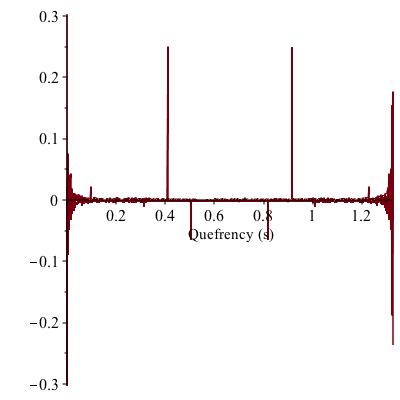 |
The cepstrum plot shows a strong peak at a quefrency of just over 0.4 s - that's probably where the echo starts. Let's find the precise location of the peak.
| > |
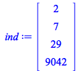 |
The peak occurs at an index of 9042. Use this information to attenuate the echo with an IIR filter
| > |
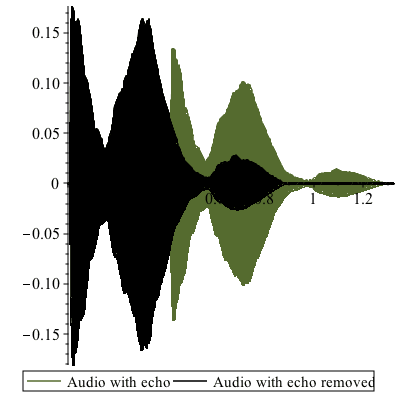
Playing the audio reveals that the echo has been attenuated
| > |
Visualize waveform of audio before and after filtering
| > |
 |
FFTShift
FFTShift swaps data in a matrix or a vector into a different position. For a matrix swapped about both dimensions, the quadrants are moved like so.
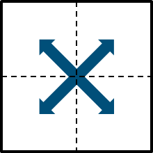
The Fourier transform of an image places lower frequency data near all four corners, with higher frequency data near the center. In this instance, FFTShift is typically applied to move the lowest frequencies to the center and the highest frequencies to the corners.
This results in a more meaningful visualization of the power spectrum where the lowest frequency data is contiguous, and simplifies the manipulation of frequency data
First, we import an image.
| > |

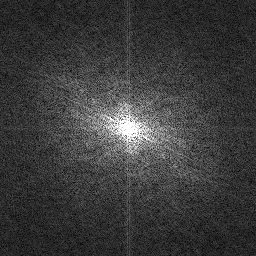
Now, we convert from the image domain to the spatial frequency domain, move the zero-frequency data to the center, and visualize the power spectrum (the square-root scaling simply rescales the frequencies for a more meaningful visualization).
| > |
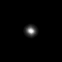
Multiply the spatial frequencies by a Gaussian mask (this is similar to a low pass filter that attenuates higher frequency data).
| > |  options operator, arrow; evalf(exp(`/`(`*`(-1, `*`(`+`(`*`(`^`(`+`(i, `-`(`*`(`/`(1, 2), `*`(nRows)))), 2)), `*`(`^`(`+...](SignalProcessing/SignalProcessing_61.gif) |
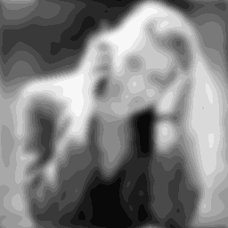
Move the zero frequency data back to their original positions, and then invert the spatial frequency data back to the image domain.
| > |
Edge Detect
The new EdgeDetect command applies an edge detection convolution mask to an image. The command supports several masks including Sobel, Robert, Prewitt 3x3 and Prewitt 4x4.
| > |

| > |

ImagePeriodogram
ImagePeriodogram calculates the magnitude of the Fourier transform of an image; this data can then be embedded as an image to visualize the spatial frequencies of the image. By default the lowest frequencies are shifted to the center (this can, however, be modified). Moreover, you can also scale the data to better visualize spatial frequencies that would otherwise not be apparent).
| > |

| > |

More Updates
Detrend
A new option for the SignalPlot, Periodogram and Spectrogram lets you remove a linear trend from the data, prior to the primary analysis.