
Maple 2019 includes a couple new plotting utilities for drawing mathematical shapes
Polygons by Name
The new command plottools[polygonbyname] draws shapes in plots. It knows about many mathematical shapes and has many options for creating them exactly as desired. This command is very useful for annotating other plots or building more complex 2-D visualizations. For example, it is used by GraphTheory[DrawGraph] to render custom vertex shapes in Graph visualizations.
| > |
The size of shapes is primarily controlled by defining the dimensions of a box that should fit entirely inside the shape. Here is a parallelogram that fits a 16x9 box.
| > |
 |
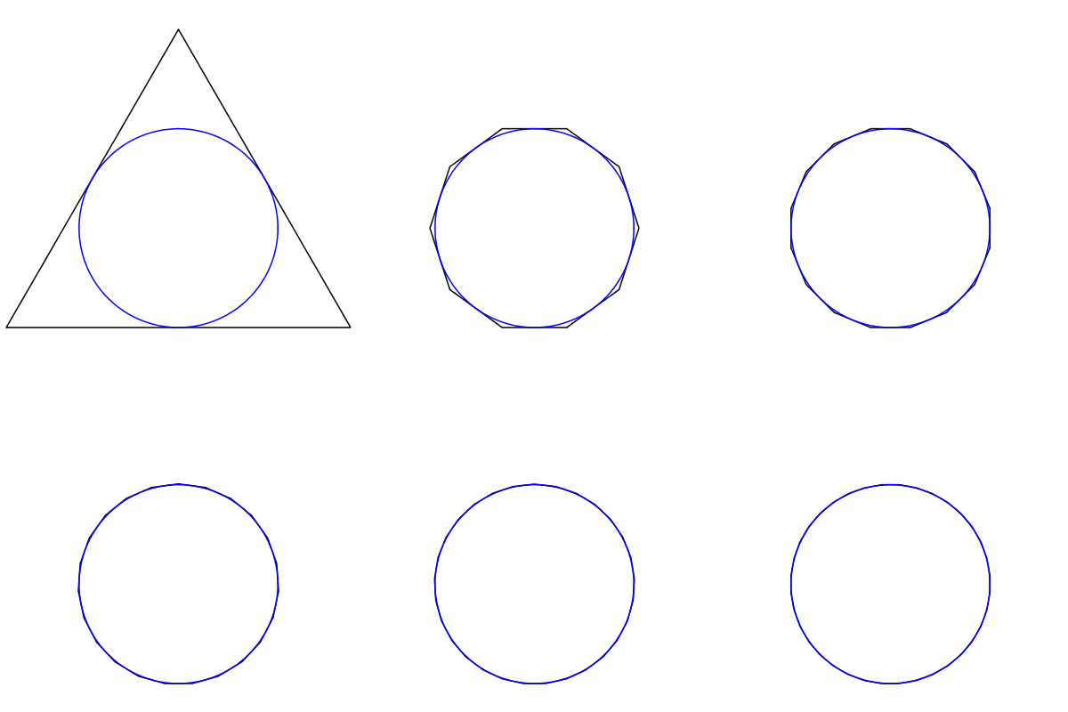
Regular polygons with an arbitrary number of sides can be specified by just a number for the name, or as "n-gon", or common name like "hexagon". Here is an animation of calling polygonbyname on the integers 3-36.
| > |
 |
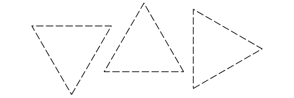
In addition to being able to specify the size of the polygon, you can specify its position with the center option and its orientation with the rotation option.
| > |
 |
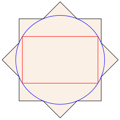
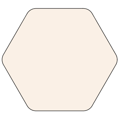
There many other ways to modify the shape with command options: irregular, reuleaux, rounded, star, and wide. Not all options, or combinations of options, are supported for every shape. See the help page for details.
| > |
| > |
 |
| > |
 |
| > |
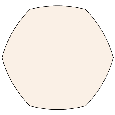 |
| > |
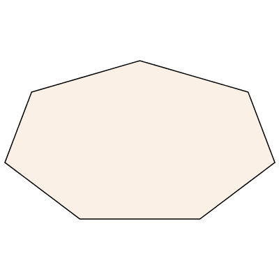 |
Most of these command options can also be specified as part of the name. Here is a wide irregular 9 pointed star.
| > |
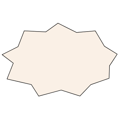 |
Many shapes commonly used in diagrams are known by name.
| > |
|
Generalized Superellipses
The plottools,ellipse and plottools,ellipticArc commands now have a super option that creates superellipses and generalized superellipses or arcs thereof. A generalized superellipse is the locus of points [x,y] satisfying the equation
![]()
for center [x0,y0], radial distances a and b, and super elliptic parameters m1 and m2. If ![]() the curve is a generalized superellipse, and just a superellipse otherwise.
the curve is a generalized superellipse, and just a superellipse otherwise.
| > |
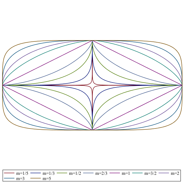 |
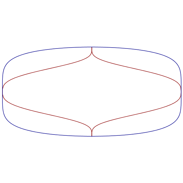
Generalized superellipses have different shapes in the x and y directions. This is most obvious when one of the parameters is less than 1 and the other is greater.
| > |
 |
Improved Visualization of Graphs
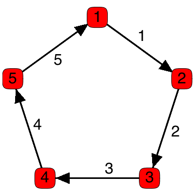
Many improvements have been made to the rendering of graphs with the DrawGraph command. As well, many new option have been added to customize the style of graphs. For full details see the GraphTheory updates page.
| > |
| > |
 |
Correlogram
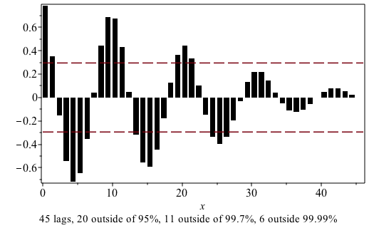
The Correlogram command in the Statistics package computes autocorrelations of a data set and displays the result as a column plot with dashed lines indicating the 95% confidence band. AutoCorrelationPlot is an alias for the Correlogram command.
| > |
 |
Animations in the Plot Builder
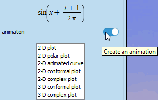
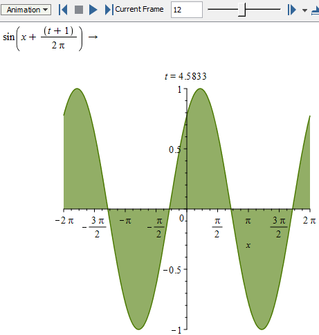
You can now build animations interactively through the Plot Builder.
Plot Export
It is now possible to export plots to the Scalable Vector Graphics (SVG) file format.