GraphTheory - New Features in Maple 2020 - Maplesoft

What's New in Maple 2020

GraphTheory

A substantial effort was put into Graph Theory for Maple 2020, including significant advances in visualization, flexible graph manipulation options, powerful analysis tools, and support for over 20 new special graphs and graph properties.

Centrality 

Maple 2020 offers eight new functions for calculating the centrality of vertices in a graph. These are: 

  • Betweenness centrality

  • Closeness centrality

  • Degree centrality

  • Eigenvector centrality

  • Harmonic centrality

  • Information centrality

  • Katz centrality

  • PageRank centrality

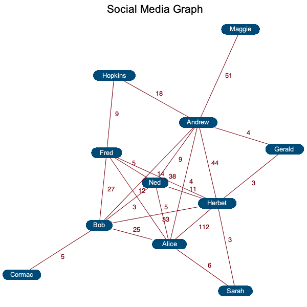
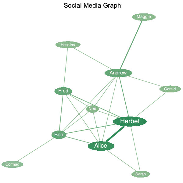
Here is an example of a simple social graph where the graph centrality measures social influence. 

> vertices := [
 

> edges_weights := {[{
edges_weights := {[{
 

> Gs := Graph(vertices, edges_weights);
 

Typesetting:-mprintslash([Gs := `Graph 1: an undirected weighted graph with 11 vertices and 22 edge(s)`], [GRAPHLN(undirected, weighted, [
 

> DrawGraph(Gs, layout = spring, stylesheet = [vertexcolor =
DrawGraph(Gs, layout = spring, stylesheet = [vertexcolor =
 

Plot_2d
 

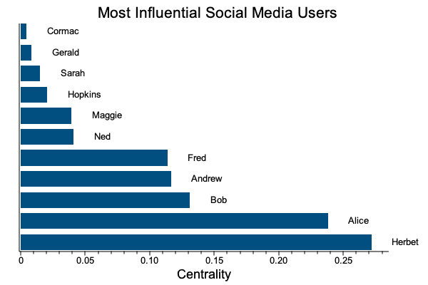
> centrality := EigenvectorCentrality(Gs);
 

Typesetting:-mprintslash([centrality := [.237978443268371, .131195758579289, .116408170276784, 0.410886760673835e-1, .113645015600347, 0.850460849139520e-2, 0.148924786849715e-1, .271820184196355, 0.4...
 

> ind := sort(centrality, `>`, output = permutation); -1
 

> Statistics:-BarChart([seq(vertices[i] = centrality[i], `in`(i, ind))], title =
Statistics:-BarChart([seq(vertices[i] = centrality[i], `in`(i, ind))], title =
 

Plot_2d
 

Graph Styling Improvements 

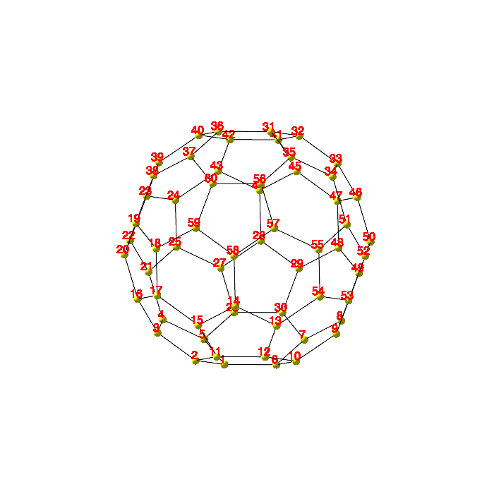
The stylesheet option to DrawGraph is now fully supported for animations and all options except the ones controlling the shapes of vertices and arrows are supported for three-dimensional graphs. 

> S := SpecialGraphs:-SoccerBallGraph(); 1

Typesetting:-mprintslash([S := `Graph 2: an undirected unweighted graph with 60 vertices and 90 edge(s)`], [GRAPHLN(undirected, unweighted, [1, 2, 3, 4, 5, 6, 7, 8, 9, 10, 11, 12, 13, 14, 15, 16, 17, ...

> DrawGraph(S, stylesheet = [vertexcolor =

Plot_2d
 

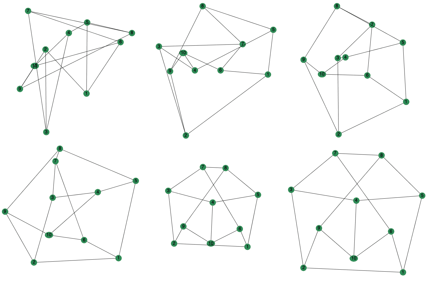
The animate option to DrawGraph can now be set to a positive integer to control the number of frames generated. 

> P := SpecialGraphs:-PetersenGraph(); 1
 

Typesetting:-mprintslash([P := `Graph 4: an undirected unweighted graph with 10 vertices and 15 edge(s)`], [GRAPHLN(undirected, unweighted, [1, 2, 3, 4, 5, 6, 7, 8, 9, 10], Array(%id = 184468839122286...
 

> DrawGraph(P, layout = spring, animate = 25, stylesheet = [vertexcolor =
 

Plot_2d
 

A few new ways to style graphs were also added. A new arrowshape style was added for directed edges allowing any shape supported by plottools. As well, the arrowpos directive has been greatly improved to be more accurate. Vertex borders can now be given a color including several special dynamic coloring options "_contrast", "_blend", and "_match" which are also supported for vertex font colors, edge color, and edge font colors. 

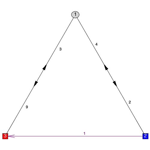
New commands have been introduced for adding styles to graph components that are independent of the concept of "highlighting". These are StyleVertex, StyleEdge, and StyleSubgraph and have basically the same calling sequences as their Highlight equivalents. They differ from their Highlight versions in that when called multiple times, they add to the existing style rather than replace it and they build on the base default style rather than the base "highlighted" style. 

> Gd := Graph(Matrix([[0, 2, 9], [4, 0, 1], [3, 0, 0]]));
 

Typesetting:-mprintslash([Gd := `Graph 5: a directed weighted graph with 3 vertices and 5 arc(s)`], [GRAPHLN(directed, weighted, [1, 2, 3], Array(%id = 18446883912228647270), `GRAPHLN/table/61`, Matri...
 

> StyleEdge(Gd, [2, 3], fontcolor =
StyleEdge(Gd, [2, 3], fontcolor =
 

> StyleVertex(Gd, 2, color =
 

> DrawGraph(Gd); 1
 

Plot_2d
 

Style Vertices and Edges by Properties 

You can now visually style graph vertices and edges with respect to properties, such as centrality or weight. For example, given its centrality, the color of a vertex can be chosen from a gradient of colors-this lets you emphasize the more important vertices in a graph. Similarly, those edges with greater weight can be assigned greater thickness.  

In this example, given the  

  • eigenvector centrality of a vertex, we linearly transition between two colors and two font sizes.

  • weight of an edge, we linearly transition between two colors and thicknesses.

> c1 :=
c1 :=
c1 :=
c1 :=
 

> DrawGraph(Gs, style = spring, stylesheet = [vertexfontcolor = white, vertexborder = false, vertexpadding = 4], title =
DrawGraph(Gs, style = spring, stylesheet = [vertexfontcolor = white, vertexborder = false, vertexpadding = 4], title =
 

Plot_2d
 

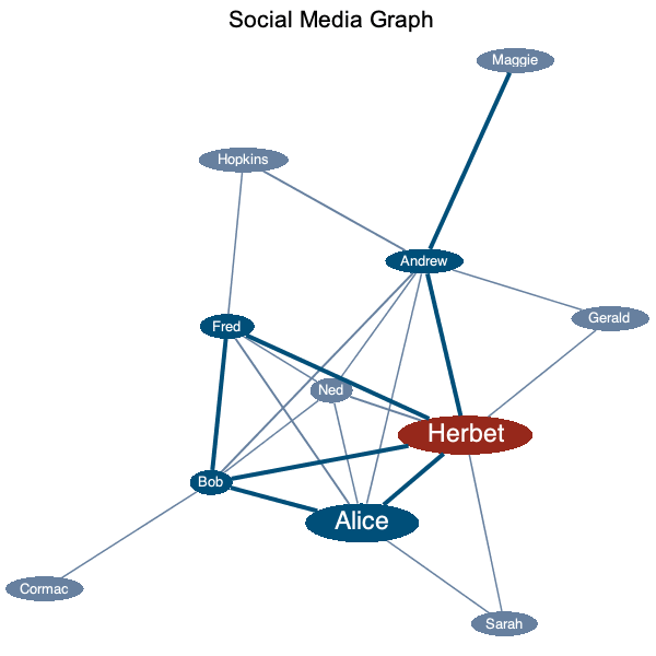
In this example, we demonstrate the valuesplit styling option that styles with a discrete set of values rather than a gradient or range: 

  • for vertices, we assign specific colors and font sizes to ranges of the eigenvector centrality.

  • for edges, we assign specific colors and thicknesses to ranges of the weight.
 

> c1 :=
c2 :=
c3 :=
StyleVerticesByProperty(Gs, EigenvectorCentrality, colorscheme = [
 

> DrawGraph(Gs, style = spring, stylesheet = [vertexfontcolor = white, vertexborder = false, vertexpadding = 4], title =
DrawGraph(Gs, style = spring, stylesheet = [vertexfontcolor = white, vertexborder = false, vertexpadding = 4], title =
 

Plot_2d
 

Graph Layout Methods 

Maple 2020 offers a number of new ways to layout plots of graphs.  The style option from previous version has been renamed layout to better clarify the difference between stylesheets and the layout of the vertices.  (The old option name style will continue to be supported as an alias for layout however).  A new option layoutoptions has been added to pass in options to layout methods to further customize them.  

> Gp := GraphTheory:-SpecialGraphs:-PetersenGraph(); 1
 

Typesetting:-mprintslash([Gp := `Graph 7: an undirected unweighted graph with 10 vertices and 15 edge(s)`], [GRAPHLN(undirected, unweighted, [1, 2, 3, 4, 5, 6, 7, 8, 9, 10], Array(%id = 18446883912192...
 

> DrawGraph(Gp, layout = spring, layoutoptions = [initial = circle, constantonly = true]); 1
 

Plot_2d
 

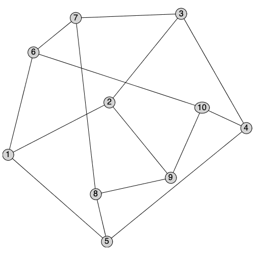
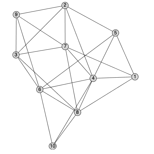
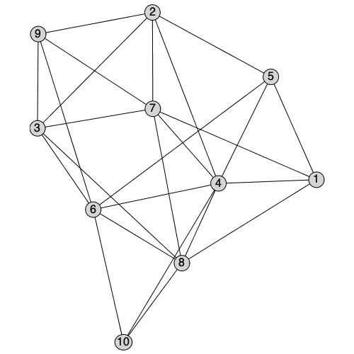
There is a new interactive method to layout graphs manually starting from a selected layout. A plot component is created where vertices can either be dragged or selected and moved to new positions. The new position will be stored as the 'user' layout, and will be the default layout for future calls to DrawGraph. 

> Gr := RandomGraphs:-RandomGraph(10, 25); 1
 

Typesetting:-mprintslash([Gr := `Graph 3: an undirected unweighted graph with 10 vertices and 25 edge(s)`], [GRAPHLN(undirected, unweighted, [1, 2, 3, 4, 5, 6, 7, 8, 9, 10], Array(1..10, {(1) = {4, 5,...
 

> DrawGraph(Gr, layout = interactive, layoutoptions = [initial = spring]);
 

Embedded component 

> DrawGraph(Gr);
 

Plot_2d


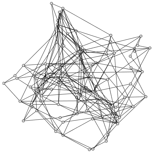
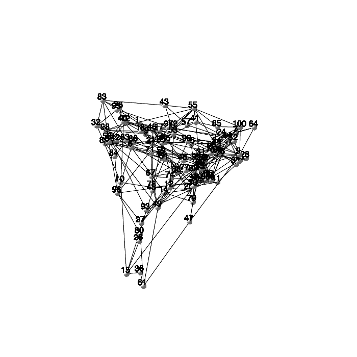
There are a few new layout methods, most notably, a new spectral two- and three-dimensional layout method. 

> G1 := RandomGraphs:-RandomGraph(100, 250);
 

Typesetting:-mprintslash([G1 := `Graph 8: an undirected unweighted graph with 100 vertices and 250 edge(s)`], [GRAPHLN(undirected, unweighted, [1, 2, 3, 4, 5, 6, 7, 8, 9, 10, 11, 12, 13, 14, 15, 16, 1...
 

> DrawGraph(G1, layout = spectral);

Plot_2d

> DrawGraph(G1, layout = spectral, dimension = 3);

Plot_2d

The grid and random layout methods are also new in Maple 2020 and support two and three dimensions.


Self-Loops 

The core routines of the GraphTheory package have been extended to support graphs with self-loops.  Graphs with self-loops may be directed or undirected, and weighted or unweighted. 

The number of self-loops in a graph is displayed in the graph description along with the vertex and edge count: 

> G := SpecialGraphs:-DeBruijnGraph(5, 3);
 

Typesetting:-mprintslash([G := `Graph 11: a directed unweighted graph with 125 vertices, 620 arc(s), and 5 self-loop(s)`], [GRAPHLN(directed, unweighted, [1, 2, 3, 4, 5, 6, 7, 8, 9, 10, 11, 12, 13, 14...
 

Several new commands have been added to work with self-loops: 

  • HasSelfLoops returns true if a graph has an edge or arc to itself.
 

  • NumberOfSelfLoops returns the number of self-loops in a graph.
 

  • SelfLoops returns the set of self-loops in a graph.
 

The HasSelfLoop and NumberOfSelfLoops commands permit querying graphs for the existence and number of self-loops, respectively, while SelfLoops returns the set of vertices with self-loops. 

> HasSelfLoop(G);
 

true
 

> NumberOfSelfLoops(G);
 

5
 

> SelfLoops(G);
 

{1, 32, 63, 94, 125}
 

Directed Graphs with Self-Loops 

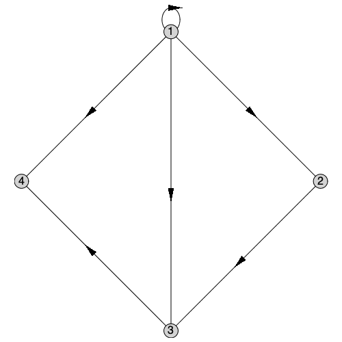
The support for self-loops extends to both directed and undirected graphs.  Here is a directed graph with a self-loop at vertex 1: 

> G1 := Graph({[1, 1], [1, 2], [1, 3], [1, 4], [2, 3], [3, 4]});
 

Typesetting:-mprintslash([G1 := `Graph 8: a directed unweighted graph with 4 vertices, 5 arc(s), and 1 self-loop(s)`], [GRAPHLN(directed, unweighted, [1, 2, 3, 4], Array(%id = 18446745818964101950), `...
 

> DrawGraph(G1);
 

Plot_2d
 

> NumberOfSelfLoops(G1);

1

The Edges command now returns self-loops in its list of edges.  If only edges between distinct vertices are desired, the option selfloops=false can be specified: 

> Edges(G1);
 

{[1, 1], [1, 2], [1, 3], [1, 4], [2, 3], [3, 4]}
 

> Edges(G1, selfloops = false);
 

{[1, 2], [1, 3], [1, 4], [2, 3], [3, 4]}
 

The in-degree and out-degree of a vertex are each increased by one when it receives a self-loop: 

> InDegree(G1, 1);
 

1
 

> OutDegree(G1, 1);
 

4
 

Undirected Graphs with Self-Loops 

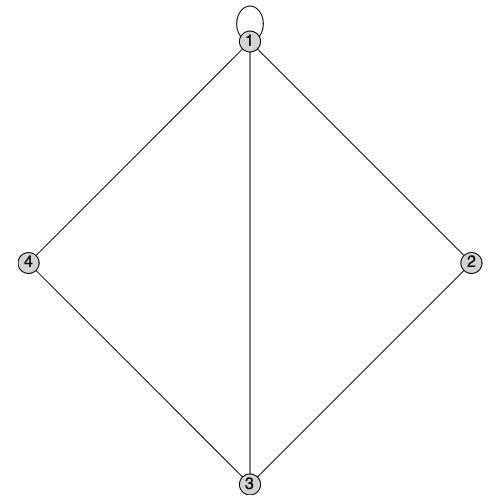
We can produce a copy of G1 which discards the directionality of its edges while preserving self-loops by calling UnderlyingGraph with the selfloops option: 

> G2 := UnderlyingGraph(G1, selfloops);
 

Typesetting:-mprintslash([G2 := `Graph 9: an undirected unweighted graph with 4 vertices, 5 edge(s), and 1 self-loop(s)`], [GRAPHLN(undirected, unweighted, [1, 2, 3, 4], Array(%id = 184467458190516504...
 

> DrawGraph(G2);
 

Plot_2d
 

By convention, the degree of a vertex is increased by 2 when it receives a self-loop: 

> DegreeSequence(G2);
 

[5, 2, 3, 2]
 

In a simple graph the smallest possible girth (length of the shortest cycle) is 3.  In a graph with a self-loop, the length of the shortest cycle is 1: 

> Girth(G2);
 

1
 

By definition, any graph with a self-loop cannot be colored with any number of colors. The chromatic polynomial therefore is identically zero: 

> ChromaticPolynomial(G2, x);
 

0
 

Removing self-loops 

We can generate a copy of a graph with the self-loops removed simply by calling UnderlyingGraph without specifying the selfloops option: 


> G3 := UnderlyingGraph(G1);
 

Typesetting:-mprintslash([G3 := `Graph 10: an undirected unweighted graph with 4 vertices and 5 edge(s)`], [GRAPHLN(undirected, unweighted, [1, 2, 3, 4], Array(%id = 18446745819051678166), `GRAPHLN/ta...
 

> NumberOfSelfLoops(G3);
 

0
 

> DegreeSequence(G3);
 

[3, 2, 3, 2]
 

> Girth(G3);
 

3
 

> ChromaticPolynomial(G3, x);
 

`*`(x, `*`(`+`(x, `-`(1)), `*`(`^`(`+`(x, `-`(2)), 2))))
 

Geometric Graphs 

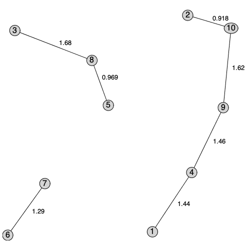
A new Maple 2020 function in RandomGraphs subpackage generates a random geometric graph. 

> G5 := RandomGraphs:-RandomGeometricGraph(10, 2, distribution = Weibull(3, 2), weighted);
 

> DrawGraph(G5);
 

Plot_2d
 

Maple 2020 contains a new subpackage, GeometricGraphs, for generating graphs from geometric data, such as a set of 2-D or 3-D points.  This subpackage includes the following new commands: 

  • DelaunayGraph
 

  • EuclideanMinimumSpanningTree
 

  • FarthestNeighborGraph
 

  • GabrielGraph
 

  • GeometricMinimumSpanningTree
 

  • NearestNeighborGraph
 

  • RelativeNeighborhoodGraph
 

  • SphereOfInfluenceGraph
 

  • UnitDiskGraph
 

  • UrquhartGraph
 

  • VisibilityGraph


> with(GeometricGraphs); 1
 

[DelaunayGraph, EuclideanMinimumSpanningTree, FarthestNeighborGraph, GabrielGraph, GeometricMinimumSpanningTree, NearestNeighborGraph, RelativeNeighborhoodGraph, SphereOfInfluenceGraph, UnitDiskGraph,...
[DelaunayGraph, EuclideanMinimumSpanningTree, FarthestNeighborGraph, GabrielGraph, GeometricMinimumSpanningTree, NearestNeighborGraph, RelativeNeighborhoodGraph, SphereOfInfluenceGraph, UnitDiskGraph,...
 

> points := Matrix(50, 2, rand(0 .. 100.)); -1


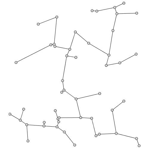
The Euclidean minimum spanning tree, the Delaunay graph, the Gabriel graph, the relative neighborhood graph, and the Urquhart graph are all derived from a Delaunay triangulation of the point data. 

These graphs have a hierarchical relationship:


  • The Euclidean minimum spanning tree is a subgraph of the relative neighborhood graph,
 

  • The relative neighborhood graph is a subgraph of the Urquhart graph,
 

  • The Urquhart graph is a subgraph of the Gabriel graph.
 

  • The Gabriel graph is a subgraph of the Delaunay graph.
 

Euclidean Minimum Spanning Tree 

Relative Neighborhood Graph 

Urquhart Graph 

Gabriel Graph 

Delaunay Graph 

DrawGraph(EuclideanMinimumSpanningTree(points));
 

Plot_2d


DrawGraph(RelativeNeighborhoodGraph(points));
 

Plot_2d


DrawGraph(UrquhartGraph(points));
 

Plot_2d


DrawGraph(GabrielGraph(points));
 

Plot_2d


DrawGraph(DelaunayGraph(points));
 

Plot_2d


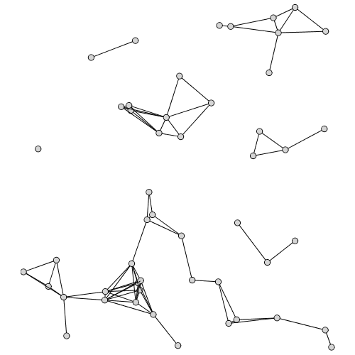
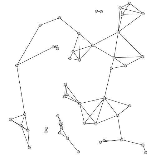
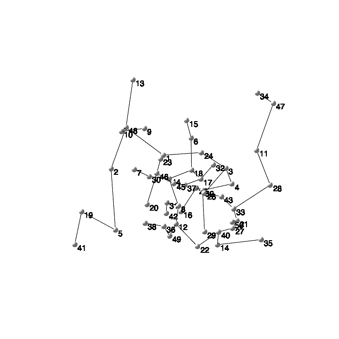
Note that we can also build spanning trees for this point data using norms other than the Euclidean norm, for example the 1-norm; the result is similar but not identical to the Euclidean spanning tree. 

DrawGraph(GeometricMinimumSpanningTree(points, 1));  

Plot_2d
 

NearestNeighborGraph and FarthestNeighborGraph return a nearest and farthest neighbor graph for a point set.  You can also build k-nearest neighbor and k-farthest neighbor graphs for specified k. 

Nearest Neighbor Graph 

Farthest Neighbor Graph 

2-Nearest Neighbor 

2-Farthest Neighbor 

DrawGraph(NearestNeighborGraph(points));
 

Plot_2d


DrawGraph(FarthestNeighborGraph(points));
 

Plot_2d


DrawGraph(NearestNeighborGraph(points, 2));
 

Plot_2d


DrawGraph(FarthestNeighborGraph(points, 2));
 

Plot_2d


The UnitDiskGraph command returns a graph in which two points are connected if their distance falls below a specified threshold. 

> DrawGraph(UnitDiskGraph(points, 15));
 

Plot_2d
 

For a set of points, SphereOfInfluenceGraph draws a circle around each point with radius equal to the distance to its nearest neighbor. The sphere of influence graph is the graph whose vertices correspond to these points in which an edge between two points exists if the corresponding circles intersect at more than one point. 

> DrawGraph(SphereOfInfluenceGraph(points));
 

Plot_2d
 

Most of these graphs commands are not limited to two dimensions, and can be used to analyze and visualize relationships with higher-dimensional data as well. 

points3D := Matrix(50, 3, rand(0 .. 100.)); -1 

DrawGraph(EuclideanMinimumSpanningTree(points3D), dimension = 3, labelstyle = offset);

Plot_2d

Split Graphs 

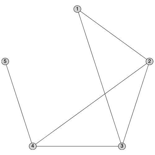
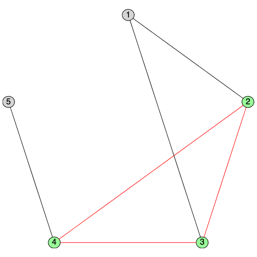
IsSplitGraph returns true if a graph is can be partitioned into a clique and an independent set. 

> G3 := Graph(5, {{1, 2}, {1, 3}, {2, 3}, {2, 4}, {3, 4}, {4, 5}}); 1; DrawGraph(G3); 1


Typesetting:-mprintslash([G3 := `Graph 12: an undirected unweighted graph with 5 vertices and 6 edge(s)`], [GRAPHLN(undirected, unweighted, [1, 2, 3, 4, 5], Array(%id = 18446745818900150742), `GRAPHLN...
Plot_2d
 

> result, split := IsSplitGraph(G3, decomposition);
 

Typesetting:-mprintslash([result, split := true, [[2, 3, 4], [1, 5]]], [true, [[2, 3, 4], [1, 5]]])
 

> HighlightSubgraph(G3, InducedSubgraph(G3, split[1]));
 

> DrawGraph(G3);
 

Plot_2d
 

ContractSubgraph 

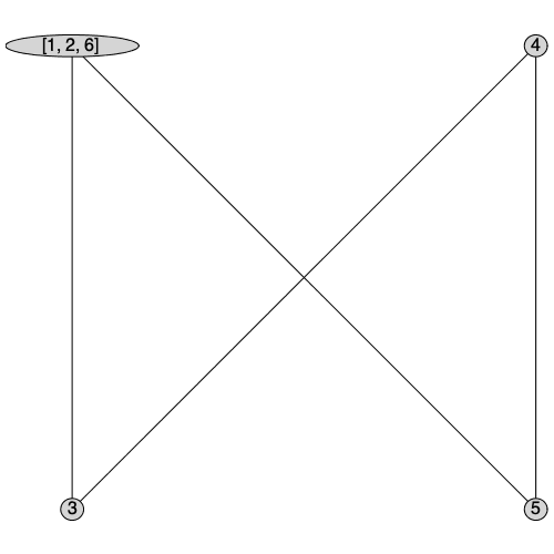
The ContractSubgraph command returns a new graph with all the vertices in S merged into a single vertex. The neighborhood of the new vertex will be the union of the neighborhoods of all of merged vertices. 

> C := CycleGraph(6); -1H := ContractSubgraph(C, [1, 2, 6]);
 

Typesetting:-mprintslash([H := `Graph 13: an undirected unweighted graph with 4 vertices and 4 edge(s)`], [GRAPHLN(undirected, unweighted, [1, 3, 4, 5], Array(%id = 18446745818914256646), `GRAPHLN/tab...
 

> DrawGraph(H);
 

Plot_2d
 

SpecialGraphs 

Maple 2020 provides support for 18 additional Special Graphs, bringing the total to 97.   

> with(SpecialGraphs); -1
 

Barnette-Bosàk-Lederberg Graph 

Berlekamp-van Lint-Seidel Graph 

Biggs-Smith Graph 

Brouwer-Haemers Graph 

> DrawGraph(BarnetteBosakLederbergGraph(), layout = planar, size = [250, 250]);
DrawGraph(BarnetteBosakLederbergGraph(), layout = planar, size = [250, 250]);
 

Plot_2d
 

> G := BerlekampVanLintSeidelGraph();
G := BerlekampVanLintSeidelGraph();
 

Typesetting:-mprintslash([G := `Graph 1: an undirected unweighted graph with 243 vertices and 2673 edge(s)`], [GRAPHLN(undirected, unweighted, [1, 2, 3, 4, 5, 6, 7, 8, 9, 10, 11, 12, 13, 14, 15, 16, 1...
 

> IsStronglyRegular(G, 'parameters');
 

true, [22, 1, 2]
 

> DrawGraph(BiggsSmithGraph(), layout = spectral, size = [250, 250]);
DrawGraph(BiggsSmithGraph(), layout = spectral, size = [250, 250]);
 

Plot_2d
 

> G := BrouwerHaemersGraph();
 

Typesetting:-mprintslash([G := `Graph 15: an undirected unweighted graph with 81 vertices and 810 edge(s)`], [GRAPHLN(undirected, unweighted, [1, 2, 3, 4, 5, 6, 7, 8, 9, 10, 11, 12, 13, 14, 15, 16, 17...
 

> IsStronglyRegular(G, 'parameters');
 

true, [20, 1, 6]
 

> ChromaticNumber(G);
 

7
 

De Bruijn Graph 

Gewirtz Graph 

Golomb Graph 

Harr Graph 

> DrawGraph(DeBruijnGraph(3, 2), size = [250, 250]);
DrawGraph(DeBruijnGraph(3, 2), size = [250, 250]);
 

Plot_2d
 

> G := GewirtzGraph();
 

Typesetting:-mprintslash([G := `Graph 16: an undirected unweighted graph with 56 vertices and 280 edge(s)`], [GRAPHLN(undirected, unweighted, [1, 2, 3, 4, 5, 6, 7, 8, 9, 10, 11, 12, 13, 14, 15, 16, 17...
 

> IsStronglyRegular(G, 'parameters');
 

true, [10, 0, 2]
 

> ChromaticNumber(G);
 

4


> DrawGraph(GolombGraph(), layout = planar, size = [250, 250]);
DrawGraph(GolombGraph(), layout = planar, size = [250, 250]);
 

Plot_2d
 

> DrawGraph(HaarGraph(7), dimension = 3, labelstyle = offset);
DrawGraph(HaarGraph(7), dimension = 3, labelstyle = offset);
 

Plot_2d
 

Harborth Graph 

Higman-Sims Graph 

M22 Graph 

McLaughlin Graph 

> DrawGraph(HarborthGraph(), layout = planar, size = [250, 250]);
DrawGraph(HarborthGraph(), layout = planar, size = [250, 250]);
 

Plot_2d
 

> G := HigmanSimsGraph();
 

Typesetting:-mprintslash([G := `Graph 17: an undirected unweighted graph with 100 vertices and 1100 edge(s)`], [GRAPHLN(undirected, unweighted, [1, 2, 3, 4, 5, 6, 7, 8, 9, 10, 11, 12, 13, 14, 15, 16, ...
 

> IsStronglyRegular(G, 'parameters');
 

true, [22, 0, 6]
 

> ChromaticNumber(G);
 

6
 

> G := M22Graph();
 

Typesetting:-mprintslash([G := `Graph 18: an undirected unweighted graph with 77 vertices and 616 edge(s)`], [GRAPHLN(undirected, unweighted, [1, 2, 3, 4, 5, 6, 7, 8, 9, 10, 11, 12, 13, 14, 15, 16, 17...
 

> IsStronglyRegular(G, 'parameters');
IsStronglyRegular(G, 'parameters');
 

true, [16, 0, 4]
 

> ChromaticNumber(G);
 

5
 

> G := McLaughlinGraph();
 

Typesetting:-mprintslash([G := `Graph 2: an undirected unweighted graph with 275 vertices and 15400 edge(s)`], [GRAPHLN(undirected, unweighted, [1, 2, 3, 4, 5, 6, 7, 8, 9, 10, 11, 12, 13, 14, 15, 16, ...
 

> IsStronglyRegular(G, parameters);
 

true, [112, 30, 56]
 

Meredith Graph 

Perkel Graph 

Rooks Graph 

Schläfli Graph 

> DrawGraph(MeredithGraph(), layout = spring, size = [250, 250]);
DrawGraph(MeredithGraph(), layout = spring, size = [250, 250]);
 

Plot_2d


> G := PerkelGraph();
 

Typesetting:-mprintslash([G := `Graph 20: an undirected unweighted graph with 57 vertices and 171 edge(s)`], [GRAPHLN(undirected, unweighted, [1, 2, 3, 4, 5, 6, 7, 8, 9, 10, 11, 12, 13, 14, 15, 16, 17...
 

> IsRegular(G);
 

true
 

> ChromaticNumber(G);
 

3
 

> DrawGraph(RooksGraph(2, 3), labelstyle = offset);
DrawGraph(RooksGraph(2, 3), labelstyle = offset);
 

Plot_2d
 

> G := SchlaefliGraph();
 

Typesetting:-mprintslash([G := `Graph 21: an undirected unweighted graph with 27 vertices and 216 edge(s)`], [GRAPHLN(undirected, unweighted, [1, 2, 3, 4, 5, 6, 7, 8, 9, 10, 11, 12, 13, 14, 15, 16, 17...
 

> IsStronglyRegular(G, 'parameters');
 

true, [16, 10, 8]
 

> ChromaticNumber(G);
 

9
 

Wells Graph 

Wiener-Araya Graph 


> DrawGraph(WellsGraph(), layout = spring, size = [250, 250]);
DrawGraph(WellsGraph(), layout = spring, size = [250, 250]);
 

Plot_2d
 

> DrawGraph(WienerArayaGraph(), layout = spring);
DrawGraph(WienerArayaGraph(), layout = spring);
 

Plot_2d