

Maple
Powerful math software that is easy to use
• Maple for Academic • Maple for Students • Maple Learn • Maple Calculator App • Maple for Industry and Government • Maple Flow • Maple for Individuals


Maple is the world leader in finding exact solutions to ordinary and partial differential equations. Maple 2020 extends that lead even further with new algorithms and techniques for solving more ODEs and PDEs, including general solutions, and solutions with initial conditions and/or boundary conditions.
For Maple 2020, there are significant improvements both in dsolve and in pdsolve for the exact solution of ODEs and PDEs, with and without initial or boundary conditions.
For ODEs, a new algorithm for computing hypergeometric solutions to 2nd order linear ODEs is capable of solving new classes of problems that were previously out of reach.
Hypergeometric solutions for second-order linear ODEs
Previous Maple releases already have algorithms for computing hypergeometric solutions for linear ODEs. The new algorithms implemented in Maple 2020, however, are more general. Suppose an ODE admits solutions of the form
![]()
where ![]() and
and ![]() are rational functions of x, and
are rational functions of x, and ![]() is the solution of some other linear ODE. Then the new algorithm can compute that other linear ODE and solve it, provided that it admits solutions of the form
is the solution of some other linear ODE. Then the new algorithm can compute that other linear ODE and solve it, provided that it admits solutions of the form
![]()
where ![]() and
and ![]() are rational functions of x,
are rational functions of x, ![]() is the hypergeomtric function and a, b, and c are arbitrary constants. The new algorithms use modular reduction, Hensel lifting, rational function reconstruction, and rational number reconstruction.
is the hypergeomtric function and a, b, and c are arbitrary constants. The new algorithms use modular reduction, Hensel lifting, rational function reconstruction, and rational number reconstruction.
This algorithm is more general than previous algorithms in that it has no restrictions neither on the degree of the pullback function ![]() nor the number of singularities of the input equation. The implementation follows the presentation by Imamoglu, E. and van Hoeij, M. "Computing Hypergeometric Solutions of Second Order Linear Differential Equations using Quotients of Formal Solutions and Integral Bases", Journal of Symbolic Computation, 83, (2017): 254-271.
nor the number of singularities of the input equation. The implementation follows the presentation by Imamoglu, E. and van Hoeij, M. "Computing Hypergeometric Solutions of Second Order Linear Differential Equations using Quotients of Formal Solutions and Integral Bases", Journal of Symbolic Computation, 83, (2017): 254-271.
Examples
A problem that admits solutions of the form ![]()
| > |
| > |  |
| > |
![y(x) = `+`(`/`(`*`(_C1, `*`(hypergeom([-`/`(1, 2), `/`(1, 2)], [1], `/`(`*`(`^`(`+`(`*`(4, `*`(x)), 1), 2)), `*`(`^`(`+`(`*`(4, `*`(x)), `-`(1)), 2)))))), `*`(`^`(x, 2))), `/`(`*`(_C2, `*`(hypergeom([...](ode-pde/PDEBC_14.gif) |
(1) |
An example where the solutions are of the form ![]()
| > |  |
| > |
| (2) |
An example with a parameter a in the coefficients
| > |
| > |
![y(x) = `+`(`/`(`*`(_C1, `*`(`^`(`+`(`*`(4, `*`(x)), `-`(3)), `/`(1, 2)), `*`(`+`(`*`(4, `*`(hypergeom([`/`(3, 2), `/`(3, 2)], [2], `+`(`*`(16, `*`(`^`(x, 2))))), `*`(x))), `-`(hypergeom([`/`(3, 2), `/...](ode-pde/PDEBC_23.gif) ![y(x) = `+`(`/`(`*`(_C1, `*`(`^`(`+`(`*`(4, `*`(x)), `-`(3)), `/`(1, 2)), `*`(`+`(`*`(4, `*`(hypergeom([`/`(3, 2), `/`(3, 2)], [2], `+`(`*`(16, `*`(`^`(x, 2))))), `*`(x))), `-`(hypergeom([`/`(3, 2), `/...](ode-pde/PDEBC_24.gif) |
(3) |
Verify this solution
| > |
| (4) |
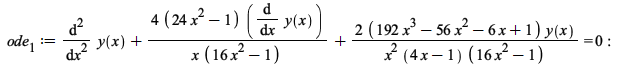
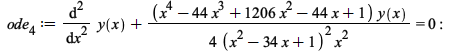
Some ODEs with 4 regular singular points that can be solved in terms of HeunG functions can also be solved using the new algorithm. This is possible whenever through a gauge transformation one of the singularities can be removed. The following ODE is of that kind, and the default solution returned by dsolve is in terms of HeunG
| > |  |
| > |
| (5) |
To get a solution in terms of hypergeometric functions you can indicate the method to be used, in this case the new method hypergeometricsols
| > |
  |
(6) |
The integrals can actually be computed
| > |
  |
(7) |
Verify this solution
| > |
| (8) |
Exact solutions to PDEs with Boundary / Initial conditions
Maple 2019 included a significant leap in the computation of exact solutions for PDE with Boundary / Initial conditions. For Maple 2020, another jump ahead in the solving capabilities happened. The examples below belong to different classes of problems out of reach of the Maple 2019 developments.
Examples
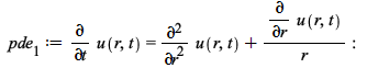
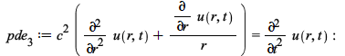
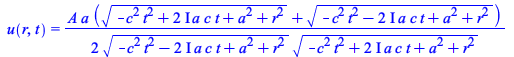
An example where the solution involves products of Bessel and Hankel functions
| > |  |
| > |
| > |
![u(r, t) = `casesplit/ans`(Sum(`+`(`-`(`/`(`*`(BesselJ(0, `*`(lambda[n], `*`(r))), `*`(Pi, `*`(`+`(`*`(BesselJ(1, lambda[n]), `*`(StruveH(0, lambda[n]))), `-`(`*`(BesselJ(0, lambda[n]), `*`(StruveH(1, ...](ode-pde/PDEBC_44.gif) |
(9) |
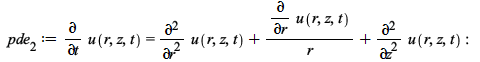
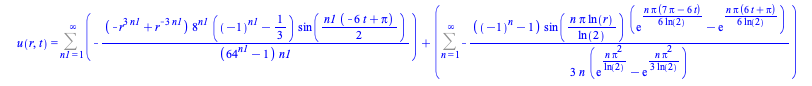
A similar problem but in three variables; the solution is a double infinite sum
| > |  |
| > |
| > |
![u(r, z, t) = `casesplit/ans`(Sum(Sum(`+`(`/`(`*`(4, `*`(BesselJ(0, `*`(lambda[n1], `*`(r))), `*`(sin(`*`(n, `*`(Pi, `*`(z)))), `*`(exp(`+`(`-`(`*`(t, `*`(`+`(`*`(`^`(Pi, 2), `*`(`^`(n, 2))), `*`(`^`(l...](ode-pde/PDEBC_48.gif) |
(10) |
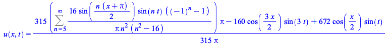
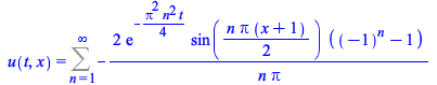
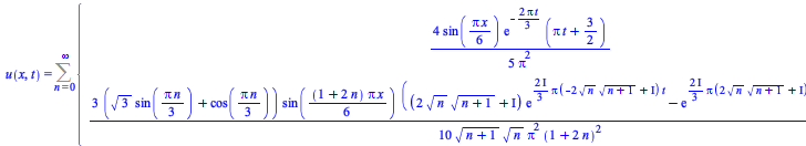
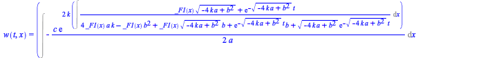
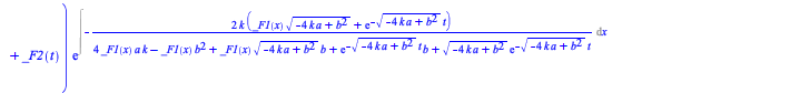
A large number of new infinite series solutions are now computable for different classes of problems (the number of boundary or initial conditions, whether they are periodic or involve derivatives of the unknown, etc.)
| > |
| > |
| > |
 |
(11) |
| > |
| > |
| > |
 |
(12) |
| > |
| > |
| > |
 |
(13) |
An example with periodic conditions in both the unknown and its first derivative, where different methods combine resulting in a solution involving an arbitrary function of x
| > |
| > |
| > |
 |
(14) |
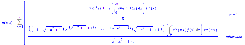
The detection of particular values of the summation index for which the solution branches with a different expression is now better:
| > |
| > |
| > |
 |
(15) |
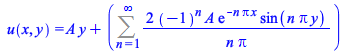
A problem with two boundary and two initial conditions, all for the unknown ![]() , where the solution method consists of splitting the problem into two PDE & BC problems and the solution is the sum of those two solutions
, where the solution method consists of splitting the problem into two PDE & BC problems and the solution is the sum of those two solutions
| > |  |
| > |
| > |
 |
(16) |
Similar example, but involving conditions for the two first derivatives of the unknown ![]()
| > |  |
| > |
| > |
 |
(17) |
A problem with initial conditions involving arbitrary functions evaluated at algebraic expressions, as ![]() , and boundary conditions that are periodic as
, and boundary conditions that are periodic as ![]()
| > |
| > |
| > |
 |
(18) |
Similar problem involving an arbitrary function in the initial conditions
| > |
| > |
| > |
 |
(19) |
Some simple, however tricky problems with nonlinear boundary conditions
| > |
| > |
| > |
| (20) |
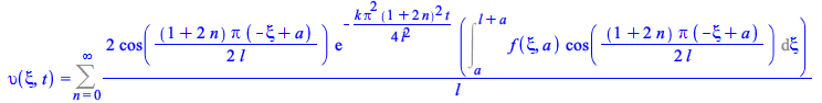
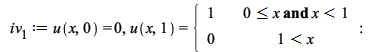
Problems with more than one evaluation point for the same variable, periodic, or involving piecewise initial conditions
| > |
| > |
| > |
 |
(21) |
| > |  |
| > | )(3, t) = 0, (D[2](u))(x, 0) = 0, u(x, 0) = piecewise(`and`(`<=`(0, x), `<=`(x, 1)), `+`(`*`(`/`(1, 10), `*`(x))), `and`(`<`(1, x), `<=`(x, 3)), `/`(1, 10)); -1](ode-pde/PDEBC_102.gif) |
| > |
  |
(22) |
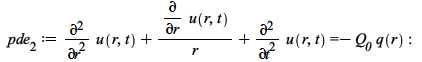
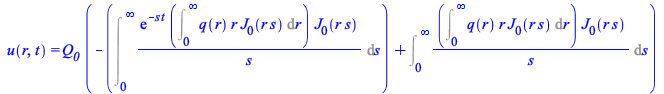
Mellin and Hankel transform solutions for PDE with Boundary Conditions
In previous Maple releases, the Fourier and Laplace transforms were used to compute exact solutions to PDE problems with boundary conditions. Now, Mellin and Hankel transforms are also used for that same purpose.
Examples:
| > |
| > |  |
| > |
| (23) |
As usual, you can let pdsolve choose the solving method, or indicate the method yourself:
| > |  |
| > |
| (24) |
It is sometimes preferable to see these solutions in terms of more familiar integrals. For that purpose, use
| > |
 |
(25) |
An example where the hankel transform is computed:
| > |  |
| > |
 |
(26) |
A general solution to a PDE calculated via rewriting the PDE as an ODE with arbitrary auxiliary functions
Under certain conditions, it is possible to rewrite a PDE as an ODE for one unknown and some auxiliary arbitrary functions. When that is possible, the solving process involves as many steps as there are independent variables in the PDE. Each step consists of solving only a single intermediate ODE (and no PDEs). In this way, a general solution is obtained for the original PDE.
Below are four examples, all of them nonlinear. For the ![]() one the solving method is shown step by step.
one the solving method is shown step by step.
Example 1:
| > |
| > |
| > |
  |
(27) |
Example 2:
| > |
| > |
| (28) |
Example 3:
| > |
| > |
| (29) |
Example 4
| > |
Step-by-step solving process for ![]()
Step 1. ![]() can be written as an ODE with respect to t by taking the derivatives of
can be written as an ODE with respect to t by taking the derivatives of ![]() with respect to x and z as auxiliary arbitrary functions of t according to
with respect to x and z as auxiliary arbitrary functions of t according to
| > |
The resulting ODE is
| > |  |
Despite the presence of the auxiliary arbitrary functions ![]() ,
, ![]() and
and ![]() , the problem is in reach of dsolve's algorithms, so solve this
, the problem is in reach of dsolve's algorithms, so solve this ![]() for
for ![]()
| > |
 |
(30) |
The solution above reduced the order of the original problem ![]() by one. Depending on the problem, more than one reduction of order may occur.
by one. Depending on the problem, more than one reduction of order may occur.
Step 2. We need to express the integration constant with respect to t in the context of a problem in t, x, and z, that is, _C1 is an arbitrary function of x and z. For illustration purposes take for instance the first solution
| > |
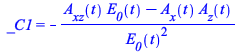 |
(31) |
| > |
 |
(32) |
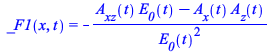
Restoring the original functions, we get
| > |
![Typesetting:-mprintslash([_F1(x, t) = `+`(`-`(`/`(`*`(`+`(`*`(diff(E(t, x, z), x, z), `*`(E(t, x, z))), `-`(`*`(diff(E(t, x, z), x), `*`(diff(E(t, x, z), z)))))), `*`(`^`(E(t, x, z), 2)))))], [_F1(x, ...](ode-pde/PDEBC_158.gif) |
(33) |
This pde in t, x, and z can now be written in terms of two auxiliary functions just of x as
| > |
Resulting in
| > | 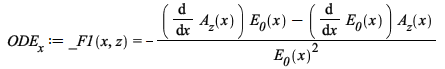 |
![Typesetting:-mprintslash([ODE__x := _F1(x, z) = `+`(`-`(`/`(`*`(`+`(`*`(diff(A__z(x), x), `*`(E__0(x))), `-`(`*`(diff(E__0(x), x), `*`(A__z(x)))))), `*`(`^`(E__0(x), 2)))))], [_F1(x, z) = `+`(`-`(`/`(...](ode-pde/PDEBC_161.gif) |
(34) |
Solve this ODE
| > |
![Typesetting:-mprintslash([E__0(x) = `/`(`*`(A__z(x)), `*`(`+`(Int(`+`(`-`(_F1(x, z))), x), _C1)))], [E__0(x) = `/`(`*`(A__z(x)), `*`(`+`(Int(`+`(`-`(_F1(x, z))), x), _C1)))])](ode-pde/PDEBC_163.gif) |
(35) |
Step 3. Proceed as in the previous step, isolating _C1 , rewriting it as an arbitrary function of z and t and restoring the original functions
| > |
![Typesetting:-mprintslash([_C1 = `+`(`-`(`/`(`*`(`+`(`*`(E__0(x), `*`(Int(`+`(`-`(_F1(x, z))), x))), `-`(A__z(x)))), `*`(E__0(x)))))], [_C1 = `+`(`-`(`/`(`*`(`+`(`*`(E__0(x), `*`(Int(`+`(`-`(_F1(x, z))...](ode-pde/PDEBC_165.gif) |
(36) |
| > |
![Typesetting:-mprintslash([_F2(t, z) = `+`(`-`(`/`(`*`(`+`(`*`(E__0(x), `*`(Int(`+`(`-`(_F1(x, z))), x))), `-`(A__z(x)))), `*`(E__0(x)))))], [_F2(t, z) = `+`(`-`(`/`(`*`(`+`(`*`(E__0(x), `*`(Int(`+`(`-...](ode-pde/PDEBC_167.gif) |
(37) |
Although not necessary, a simplification is possible in that the integral of an arbitrary function is also an arbitrary function, so we can remove the integration by redefining ![]()
| > |
| (38) |
Restore the original variables
| > |
![Typesetting:-mprintslash([_F2(t, z) = `+`(`-`(`/`(`*`(`+`(`-`(`*`(E(t, x, z), `*`(_F1(x, z)))), `-`(diff(E(t, x, z), z)))), `*`(E(t, x, z)))))], [_F2(t, z) = `+`(`-`(`/`(`*`(`+`(`-`(`*`(E(t, x, z), `*...](ode-pde/PDEBC_172.gif) |
(39) |
This resulting pde is already an ODE in disguise, from where the general solution to the original problem ![]() is
is
| > |
| (40) |
This solution can be simplified further by redefining ![]() and
and ![]()
| > |
| (41) |
Verify this solution with the original ![]()
| > |
| (42) |
Doing all these steps in one go
| > |
| (43) |
Solving a PDE by making use of first integrals
Any PDE can be solved iterating the two steps below related to its first integrals, when they can be computed.
Step 1: Write the differential equation for a first integral - a function ![]() of the PDE's jet space - by equating to 0 its total derivative with respect to (any) one of the independent variables of the original problem. The resulting PDE is of first order and can be tackled using the characteristic strip method.
of the PDE's jet space - by equating to 0 its total derivative with respect to (any) one of the independent variables of the original problem. The resulting PDE is of first order and can be tackled using the characteristic strip method.
Step 2: When the PDE for ![]() can be solved, the solution is an arbitrary function of the differential invariants of the PDE for
can be solved, the solution is an arbitrary function of the differential invariants of the PDE for ![]() . Equate one such differential invariant to an arbitrary function of the remaining independent variables of the problem, resulting in a pde of reduced order with respect to the original PDE problem, a first integral. At this point one can either repeat the process to calculate more first integrals in order to attempt an algebraic elimination (multiple reduction of order) or move again to Step 1 with the reduced order PDE.
. Equate one such differential invariant to an arbitrary function of the remaining independent variables of the problem, resulting in a pde of reduced order with respect to the original PDE problem, a first integral. At this point one can either repeat the process to calculate more first integrals in order to attempt an algebraic elimination (multiple reduction of order) or move again to Step 1 with the reduced order PDE.
Examples
| > |
| > |
| > |
| (44) |
| > |
| (45) |
| > |
| (46) |
The solving process step-by-step
Construct an expression for the first integral ![]() , where
, where ![]() , the jet space of
, the jet space of ![]()
| > |
| (47) |
| > |
| (48) |
Take the total derivative of ![]() with respect to x
with respect to x
| > |
| (49) |
Take this PDE modulo ![]() , and that is all the formulation of the problem
, and that is all the formulation of the problem
| > |
| (50) |
| > |
| (51) |
Solve ![]() , and in doing so, the solution cannot depend on
, and in doing so, the solution cannot depend on ![]() (it can only depend on
(it can only depend on ![]() . You can achieve that using the ivars option of pdsolve
. You can achieve that using the ivars option of pdsolve
| > |
| (52) |
Since ![]() is a first integral, the arguments of the arbitrary function entering this solution are also first integrals. Take the second one, which involves 1st order derivatives, and equate it to an arbitrary function all the independent variables but x (the variable used when taking the total derivative of
is a first integral, the arguments of the arbitrary function entering this solution are also first integrals. Take the second one, which involves 1st order derivatives, and equate it to an arbitrary function all the independent variables but x (the variable used when taking the total derivative of ![]() . In this case, there is only one other variable, y.
. In this case, there is only one other variable, y.
| > |
| (53) |
Rewrite this result in function notation
| > |
| (54) |
This result is already an ODE in disguise; solve it to arrive at the general solution of ![]()
| > |
| (55) |
A more involved example:
| > |
| > |
 |
(56) |
Verify this solution
| > |
| (57) |
PDE parameterized symmetries
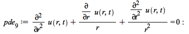
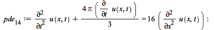
The determination of symmetries for partial differential equation systems (PDE) is relevant in several contexts, the most obvious of which is of course the determination of the PDE solutions. For instance, generally speaking, the knowledge of a N-dimensional Lie symmetry group can be used to reduce the number of independent variables of PDE by N. So if PDE depends only on N independent variables, that amounts to completely solving it. If only N-1 symmetries are known or can be successfully used then PDE becomes an ODE; and so on. In Maple, a complete set of symmetry commands, to perform each step of the symmetry approach or several of them in one go, are part of the PDEtools package.
Besides the dependent and independent variables, PDE frequently depends on some constant parameters. One can compute the PDE symmetries for arbitrary values of those parameters, but for some particular values PDE may transform into a different problem, admitting different symmetries. The question then is: how can you determine those particular values of the parameters and the corresponding different symmetries?
In connection, in Maple 2020, the computation of parameterized symmetries, whether the parameters are taken as continuous or not, can be done automatically. In what follows, first the problems and the solving approach are presented, then it is shown how they can be tackled in one go using Infinitesimals and DeterminingPDE and their new options for handling parameterized symmetries.
Consider the family of Korteweg-de Vries equations for ![]() involving three constant parameters
involving three constant parameters ![]() . For convenience (simpler input and more readable output) use the diff_table and declare commands:
. For convenience (simpler input and more readable output) use the diff_table and declare commands:
| > |
| > |
| > |
| > |
| (58) |
| > |
| (59) |
This ![]() admits a 4-dimensional symmetry group, whose infinitesimals - for arbitrary values of the parameters
admits a 4-dimensional symmetry group, whose infinitesimals - for arbitrary values of the parameters ![]() - are given by
- are given by
| > |
| (60) |
Looking at ![]() as a nonlinear problem in u, a, b and q, it splits into four cases for some particular values of the parameters:
as a nonlinear problem in u, a, b and q, it splits into four cases for some particular values of the parameters:
| > |
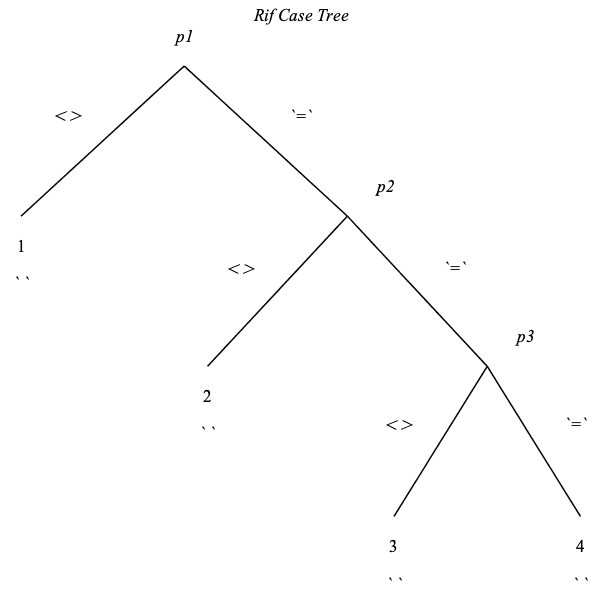 |
|
| (61) |
The legend above indicates the pivots and the tree of cases, depending on whether each pivot is equal or different from 0, followed by the algebraic sequence of cases.
The first case is the general case, for which the symmetry infinitesimals were computed in (60) ![]() , but clearly the other three cases admit more general symmetries. Consider for instance the second case, use
, but clearly the other three cases admit more general symmetries. Consider for instance the second case, use ![]() to ignore the parameterizing equation
to ignore the parameterizing equation ![]() when computing the determining PDE for the infinitesimals, and you get
when computing the determining PDE for the infinitesimals, and you get
| > |
   |
(62) |
These infinitesimals are clearly more general than ![]() , in fact so general that (62) is almost unreadable. Specialize the three arbitrary functions into something "easy" just to be able to follow - e.g. take _F1 to be the + operator, _F2 = *, and
, in fact so general that (62) is almost unreadable. Specialize the three arbitrary functions into something "easy" just to be able to follow - e.g. take _F1 to be the + operator, _F2 = *, and ![]()
| > |
 |
(63) |
| > |
| (64) |
As expected, these infinitesimals are different than the ones computed for the general case in (60).
The symmetry (64) can be verified against ![]() or directly against pde after substituting
or directly against pde after substituting ![]() .
.
| > |
| (65) |
| > |
| (66) |
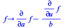
New in Maple 2020, the computation of symmetries parameterized by a, b and q, derived step-by-step in (62), can now be performed in one go by indicating the parameters (regarding the option ![]() , see the next section)
, see the next section)
| > |
    |
(67) |
In this result, the second list is the one obtained step-by-step in (62).
Parameter-continuous symmetry transformations
A different, however closely related question, is whether pde admits "symmetries with respect to the parameters a, b and q", so whether there exist continuous transformations of the parameters a, b and q that leave pde invariant in form.
Note that since the parameters are constants with regards to the dependent and independent variables (in this example ![]() ), such continuous symmetry transformations cannot be used directly to compute a solution for pde. They can, however, be used to reduce the number of parameters. And in some contexts, that is exactly what we need, for example to entirely remove the splitting into cases due to their presence, or to apply a solving method that is valid only when there are no parameters (frequently the case when computing exact solutions to PDEs with boundary conditions).
), such continuous symmetry transformations cannot be used directly to compute a solution for pde. They can, however, be used to reduce the number of parameters. And in some contexts, that is exactly what we need, for example to entirely remove the splitting into cases due to their presence, or to apply a solving method that is valid only when there are no parameters (frequently the case when computing exact solutions to PDEs with boundary conditions).
In connection, in Maple 2020, the computation of the infinitesimals that lead to parameter continuous symmetry transformations, is now automatic when you request that. As in the previous section, first the problem is presented and at the end of the section the new functionality is illustrated solving the problem in one go.
To compute such "continuous symmetry transformations of the parameters" that leave pde invariant, one can always think of these parameters as "additional independent variables of pde". In terms of formulation, that amounts to replacing the dependency in the dependent variables, in this example replacing ![]() by
by ![]()
| > |
| (68) |
| > |
| (69) |
Compute the infinitesimals for ![]() , for readability, avoid displaying the redundant functionality
, for readability, avoid displaying the redundant functionality ![]() on the left-hand sides
on the left-hand sides
| > |
| (70) |
Comparing with (60), this list of infinitesimals includes three additional ones, related to continuous transformations of ![]() and
and ![]() . This result is more general than what is convenient for algebraic manipulations, so specialize the seven arbitrary functions of
. This result is more general than what is convenient for algebraic manipulations, so specialize the seven arbitrary functions of ![]() and keep only the first symmetry that results from this specialization: that suffices to illustrate the removal of any of the three parameters a, b, and q
and keep only the first symmetry that results from this specialization: that suffices to illustrate the removal of any of the three parameters a, b, and q
| > |
| (71) |
To remove the parameters, as is standard in the symmetry approach, compute a transformation to canonical coordinates, with respect to the parameter a. That means a transformation that changes the list of infinitesimals, or likewise its infinitesimal generator representation,
| > |
 |
(72) |
into ![]() , or its equivalent generator representation
, or its equivalent generator representation ![]() . That same transformation, when applied to
. That same transformation, when applied to ![]() , entirely removes the parameter a.
, entirely removes the parameter a.
The transformation is computed using CanonicalCoordinates and the last argument indicates the "independent variable" (in our case a parameter) that the transformation should remove. We choose to remove the parameter a:
| > |
| (73) |
| > |
| (74) |
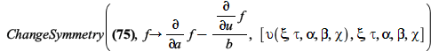
Invert this transformation in order to apply it
| > |
| (75) |
The next step is not necessary, but just to understand how all this works, verify the effect of this transformation on the infinitesimal generator 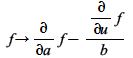
| > |  |
| (76) |
Now that we see the transformation (75) is the one we want, use it to change variables in ![]()
| > |
| (77) |
As expected, this result depends only on two parameters, ![]() , and
, and ![]() , and the one equivalent to a (that is
, and the one equivalent to a (that is ![]() , see the transformation used (75)), is not present anymore.
, see the transformation used (75)), is not present anymore.
To remove b or q we use the same steps, (73), (75) and (77), just changing the parameter to be removed, indicated as the last argument in the call to CanonicalCoordinates. For example, to eliminate b (represented in the new variables by ![]() ), input
), input
| > |
| (78) |
| > |
| (79) |
| > |
| (80) |
and as expected this result does not contain ![]() To remove a second parameter, the whole cycle is repeated starting with computing infinitesimals, for instance for (80).
To remove a second parameter, the whole cycle is repeated starting with computing infinitesimals, for instance for (80).
The computation of continuous transformations of the parameters a, b and q that leave pde invariant in form, done above step-by-step starting at equation (70), useful to remove parameters from the differential equation system, can now be performed in one go by indicating the parameters to Infinitesimals, and that these are to be taken as continuous:
| > |
 |
(81) |
In this result, the first infinitesimal is actually that of equation (70).


