Physics - New Features in Maple 2020 - Maplesoft

What's New in Maple 2020

Physics

Maple provides a state-of-the-art environment for algebraic computations in Physics, with emphasis on ensuring that the computational experience is as natural as possible. The theme of the Physics project for Maple 2020 has been the consolidation of the functionality introduced in previous releases, together with significant enhancements to further strengthen the functionality especially in:

  • Particle Physics: the Scattering matrix in coordinates and momentum representation and related Feynman Diagrams,
  • General Relativity: the slicing and spatial gauge conditions of the 3+1 decomposition of spacetime, and numerical relativity
  • The connection between different tensors and related differentiation operations
  • Simplification of tensorial expressions, now involving spinor, su2 and su3 tensor indices


Overall, the enhancements throughout the entire package further extend the range of Physics-related algebraic computations that can be done naturally in a worksheet. The presentation below illustrates both the novelties and the kind of mathematical formulations that can now be performed.
 

As part of its commitment to providing the best possible environment for algebraic computations in Physics, Maplesoft launched a Maple Physics: Research and Development website in 2014, which enabled users to download research versions, ask questions, and provide feedback. The results from this accelerated exchange with people around the world have been incorporated into the Physics package in Maple 2020.


Feynman Diagrams - the scattering matrix in coordinates and momentum representation

  • In connection, for Maple 2020 a full rewriting of the FeynmanDiagrams command, now including a myriad of new capabilities (mainly a. b. and c. and related options - see below), reversing the previous status of things entirely.

  • A scattering matrix relates the initial and final states, `#mfenced(mrow(mo( and `#mfenced(mrow(mo(, of a quantum interacting system. In a 4-dimensional spacetime with coordinates X; , S; can be written as:

S = T(exp(`*`(i, `*`(`#mrow(mo( 

  • where i; is the imaginary unit and L; is the interaction Lagrangian, written in terms of quantum fields depending on the spacetime coordinates X; . The T symbol means time-ordered. For the terminology used in this page, see for instance chapter IV, "The Scattering Matrix", of ref.[1].

  • This exponential can be expanded as
 

S = `+`(1, S[1], S[2], S[3], `...`);  

  • where

S[n] = `#mrow(mo( 

  • and T(L(X[1]), `...`, L(X[n])); is the time-ordered product of n interaction Lagrangians evaluated at different points. The S matrix formulation is at the core of perturbative approaches in relativistic Quantum Field Theory, where exact solutions are known only for some 2-dimensional models.

  • In brief, the new functionality includes computing:

  • The expansion S = `+`(1, S[1], S[2], S[3], `...`); in coordinates representation up to arbitrary order (the limitation is now only the hardware)

  • The S-matrix element `#mfenced(mrow(mo( in momentum representation up to arbitrary order for given number of loops and initial and final particles (the contents of the `#mfenced(mrow(mo( and `#mfenced(mrow(mo( states); optionally, also the transition probability density, constructed using the square of the scattering matrix element `*`(`^`(abs(`#mfenced(mrow(mo(, as shown in formula (13) of sec. 21.1 of ref.[1].

  • The Feynman diagrams (drawings) related to the different terms of the expansion of S or of its matrix elements `#mfenced(mrow(mo(.

  • Interaction Lagrangians involving derivatives of fields, typically appearing in non-Abelian gauge theories, are handled, and several options are provided enabling restricting the outcome regarding the incoming and outgoing particles, the number of loops, vertices or external legs, the propagators and normal products, or whether to compute tadpoles and 1-particle reducible terms.
 

Examples 

For illustration purposes set three coordinate systems, and set phi; to represent a quantum operator 

> with(Physics); -1

> Setup(mathematicalnotation = true, coordinates = [X, Y, Z], quantumoperators = phi);


`*`(`Systems of spacetime coordinates are:`, `*`({X = (x1, x2, x3, x4), Y = (y1, y2, y3, y4), Z = (z1, z2, z3, z4)}));
_______________________________________________________;
[coordinatesystems = {X, Y, Z}, mathematicalnotation = true, quantumoperators = {phi}] (1)
 

Let L; be the interaction Lagrangian 

> L := `*`(lambda, `*`(`^`(phi(X), 4)));

Typesetting:-mprintslash([L := `*`(lambda, `*`(Physics:-`^`(phi(X), 4)))], [`*`(lambda, `*`(Physics:-`^`(phi(X), 4)))]) (2)
 

The expansion of S; in coordinates representation, computed by default up to order = 3 (you can change that using the option order = n), by definition containing all possible configurations of external legs, displaying the related Feynman Diagrams, is given by 

> %eval(S, `=`(order, 3)) = FeynmanDiagrams(L, diagrams);

Plot_2d Plot_2d Plot_2d

Typesetting:-mrow(Typesetting:-mrow(Typesetting:-mi(
(3)

The expansion of S;  in coordinates representation to a specific order shows in a compact way the topology of the underlying Feynman diagrams. Each integral is represented with a new command, FeynmanIntegral, that works both in coordinates and momentum representation. To each term of the integrands corresponds a diagram, and the correspondence is always clear from the symmetry factors and normal products shown.  

In a typical situation, one wants to compute a specific term, or scattering process, instead of the S matrix up to some order with all possible configurations of external legs. For example, to compute only the terms of this result above that correspond to diagrams with 1 loop use numberofloops = 1 (for tree-level, use numberofloops = 0)

> %eval(S, [`=`(order, 3), `=`(loops, 1)]) = FeynmanDiagrams(L, numberofloops = 1, diagrams);

Plot_2d Plot_2d

Typesetting:-mrow(Typesetting:-mrow(Typesetting:-mi(
(4)
 

In the result above there are two terms, with 4 and 6 external legs respectively.  

A scattering process with matrix element `#mfenced(mrow(mo( in momentum representation, corresponding to the term with 4 external legs (symmetry factor = 72), could be any process where the total number of incoming + outgoing particles is equal to 4. For example, one with 2 incoming and 2 outgoing particles. The transition probability for that process is given by 

> %eval(`#mfenced(mrow(mo(

Plot_2d
Typesetting:-mrow(Typesetting:-mrow(Typesetting:-mi(
(5)
 

When computing in momentum representation, only the topology of the corresponding Feynman diagrams is shown (i.e. the diagrams associated to the corresponding Feynman integral in coordinates representation). 

The transition matrix element `#mfenced(mrow(mo( is related to the transition probability density dw; (formula (13) of sec. 21.1 of ref.[1]) by


dw = `*`(`^`(`+`(`*`(2, `*`(Pi))), `+`(`*`(3, `*`(s)), `-`(4))), `*`(n__1, `*`(`...`, `*`(n__s, `*`(`^`(abs(F(p[i], p[f])), 2), `*`(delta(`+`(sum(p[i], i = 1 .. s), `-`(sum(p[f], f = 1 .. r)))), `*`(`...


where `*`(n__1, `*`(`...`, `*`(n__s))); represent the particle densities of each of the s particles in the initial state `#mfenced(mrow(mo(, the delta; (Dirac) is the expected singular factor due to the conservation of the energy-momentum and the amplitude F(p[i], p[f]); is related to `#mfenced(mrow(mo( via 

`#mfenced(mrow(mo(


To directly get the probability density dw; instead of`#mfenced(mrow(mo(use the option output = probabilitydensity 

> FeynmanDiagrams(L, incomingparticles = [phi, phi], outgoingparticles = [phi, phi], numberofloops = 1, output = probabilitydensity);
 

Typesetting:-mrow(Typesetting:-mrow(Typesetting:-mi( (6)

In practice, the most common computations involve processes with 2 or 4 external legs. To restrict the expansion of the scattering matrix in coordinates representation to that kind of processes use the numberofexternallegs option. For example, the following computes the expansion of S; up to order = 3, restricting the outcome to the terms corresponding to diagrams with only 2 external legs 

> %eval(S, [`=`(order, 3), `=`(legs, 2)]) = FeynmanDiagrams(L, numberofexternallegs = 2, diagrams);


Plot_2d Plot_2d Plot_2d

Typesetting:-mrow(Typesetting:-mrow(Typesetting:-mi(
(7)
 

This result shows two Feynman integrals, with respectively 2 and 3 loops, the second integral with two terms. The transition probability density in momentum representation for the process %Bracket(phi, S, phi); corresponding to the first integral (1 term with symmetry factor = 96) is then 

> FeynmanDiagrams(L, incomingparticles = [phi], outgoingparticles = [phi], numberofloops = 2, diagrams, output = probabilitydensity);


Plot_2d

Typesetting:-mrow(Typesetting:-mrow(Typesetting:-mi(
(8)
 

In the above, for readability, the contracted spacetime indices in the square of momenta entering the amplitude F (as denominators of propagators) are implicit. To make those indices explicit, use the option putindicesinsquareofmomentum 

> %eval(%Bracket(phi, S, phi), `=`(loops, 2)) = FeynmanDiagrams(L, incoming = [phi], outgoing = [phi], numberofloops = 2, indices);

`*`(`* Partial match of  '`, `*`(indices, `*`(`' against keyword '`, `*`(putindicesinsquareofmomentum, `*`(`' `)))));
Typesetting:-mrow(Typesetting:-mrow(Typesetting:-mi(
(9)
 

This computation can also be performed to higher orders. For example, with 3 loops, in coordinates and momentum representations, corresponding to the other two terms and diagrams in (7) 

> %eval(S[3], [`=`(legs, 2), `=`(loops, 3)]) = FeynmanDiagrams(L, legs = 2, loops = 3);


`*`(`* Partial match of  '`, `*`(legs, `*`(`' against keyword '`, `*`(numberoflegs, `*`(`' `)))));
`*`(`* Partial match of  '`, `*`(loops, `*`(`' against keyword '`, `*`(numberofloops, `*`(`' `)))));
Typesetting:-mrow(Typesetting:-mrow(Typesetting:-mi(
(10)
 

> %eval(%Bracket(phi, S, phi), `=`(loops, 3)) = FeynmanDiagrams(L, incomingparticles = [phi], outgoingparticles = [phi], numberofloops = 3);
 

Typesetting:-mrow(Typesetting:-mrow(Typesetting:-mi(
(11)
 

Consider the interaction Lagrangian of Quantum Electrodynamics (QED). To formulate the problem start defining the vector field A[mu]; . 

> Define(A[mu]);

`Defined objects with tensor properties`;
Typesetting:-mprintslash([[A[mu], Physics:-Dgamma[mu], P__1[mu], P__2[mu], P__3[mu], P__4[mu], Physics:-Psigma[mu], Physics:-d_[mu], Physics:-g_[mu, nu], p__1[mu], p__2[mu], p__3[mu], p__4[mu], p__5[m... (12)
 

Set lowercase Latin letters from i to s to represent spinor indices (you can change this setting according to your preference using Setup), also the (anticommutative) spinor field will be represented below by psi; , so set psi; as an anticommutativeprefix, and set A; and psi; as quantum operators 

> Setup(spinorindices = lowercaselatin_is, anticommutativeprefix = psi, op = {A, psi});


`*`(`* Partial match of  '`, `*`(op, `*`(`' against keyword '`, `*`(quantumoperators, `*`(`' `)))));
_______________________________________________________;
[anticommutativeprefix = {psi}, quantumoperators = {A, phi, psi}, spinorindices = lowercaselatin_is] (13)

The matrix indices of the Dirac matrices are written explicitly and use conjugate to represent the Dirac conjugate conjugate(psi[j]);

> L__QED := `*`(alpha, `*`(conjugate(psi[j](X)), `*`(Dgamma[mu][j, k], `*`(psi[k](X), `*`(A[mu](X))))));

Typesetting:-mprintslash([L__QED := `*`(alpha, `*`(Physics:-`*`(conjugate(psi[j](X)), psi[k](X), A[mu](X)), `*`(Physics:-Dgamma[`~mu`][j, k])))], [`*`(alpha, `*`(Physics:-`*`(conjugate(psi[j](X)), psi... (14)
 

Compute S[2]; , only the terms with 4 external legs, and display the diagrams: they have no loops 

> %eval(S[2], `=`(legs, 4)) = FeynmanDiagrams(L__QED, numberofvertices = 2, numberoflegs = 4, diagrams);
 

Plot_2d Plot_2d

Typesetting:-mrow(Typesetting:-mrow(Typesetting:-mi(
(15)
 

The same computation but with only 2 external legs results in the diagrams with 1 loop that correspond to the self-energy of the electron and the photon (page 218 of ref.[1])

> %eval(S[2], `=`(legs, 2)) = FeynmanDiagrams(L__QED, numberofvertices = 2, numberoflegs = 2, diagrams);

Plot_2d Plot_2d

Typesetting:-mrow(Typesetting:-mrow(Typesetting:-mi(
(16)
 

where the diagram with two spinor legs is the electron self-energy.  


To restrict the output furthermore, for example getting only the self-energy of the photon, you can specify the
normal products you want: 

> %eval(S[2], [`=`(legs, 2), `=`(products, _NP(A, A))]) = FeynmanDiagrams(L__QED, numberofvertices = 2, numberoflegs = 2, normalproduct = _NP(A, A));

`*`(`* Partial match of  '`, `*`(normalproduct, `*`(`' against keyword '`, `*`(normalproducts, `*`(`' `)))));
Typesetting:-mrow(Typesetting:-mrow(Typesetting:-mi( (17)
 

The corresponding S-matrix elements in momentum representation 

> %eval(%Bracket(A, S, A), `=`(loops, 1)) = FeynmanDiagrams(L__QED, incomingparticles = [A], outgoing = [A], numberofloops = 1, diagrams);


Plot_2d

Typesetting:-mrow(Typesetting:-mrow(Typesetting:-mi(
(18)
 

where varepsilon[A]; is the corresponding polarization vector. 

The self-energy of the electron: 

> %eval(%Bracket(psi, S, psi), `=`(loops, 1)) = FeynmanDiagrams(L__QED, incoming = [psi], outgoing = [psi], numberofloops = 1);
 

Typesetting:-mrow(Typesetting:-mrow(Typesetting:-mi(
(19)
 

In this result we see the u[psi]; spinor (see ref.[2]), and the propagator of the field A[mu]; with a mass m[A]; . To indicate that this field is massless use 

> Setup(massless = A);

`*`(`* Partial match of  '`, `*`(massless, `*`(`' against keyword '`, `*`(masslessfields, `*`(`' `)))));
_______________________________________________________;
[masslessfields = {A}] (20)
 

Now the propagator for A[mu]; is the one of a massless vector field: 

> %eval(%Bracket(psi, S, psi), `=`(loops, 1)) = FeynmanDiagrams(L__QED, incoming = [psi], outgoing = [psi], numberofloops = 1);
 

Typesetting:-mrow(Typesetting:-mrow(Typesetting:-mi( (21)
 

When working with non-Abelian gauge fields, the interaction Lagrangian involves derivatives. FeynmanDiagrams can handle that kind of interaction in momentum representation. Consider for instance a Yang-Mills theory with a massless field B[mu, a]; where a is a SU2 index (see eq.(12) of sec. 19.4 of ref.[1]). The interaction Lagrangian can be entered as follows 

> Setup(su2indices = lowercaselatin_ah, massless = B, op = B);


`*`(`* Partial match of  '`, `*`(massless, `*`(`' against keyword '`, `*`(masslessfields, `*`(`' `)))));
`*`(`* Partial match of  '`, `*`(op, `*`(`' against keyword '`, `*`(quantumoperators, `*`(`' `)))));
_______________________________________________________;
[masslessfields = {A, B}, quantumoperators = {A, B, phi, psi, psi1}, su2indices = lowercaselatin_ah] (22)
 

> Define(B[mu, a], quiet); -1
 

> F__B[mu, nu, a] := `+`(d_[mu](B[nu, a](X)), `-`(d_[nu](B[mu, a](X))));


Typesetting:-mprintslash([F__B[mu, nu, a] := `+`(Physics:-d_[mu](B[nu, a](X), [X]), `-`(Physics:-d_[nu](B[mu, a](X), [X])))], [`+`(Physics:-d_[mu](B[nu, a](X), [X]), `-`(Physics:-d_[nu](B[mu, a](X), [... (23)
> L := `+`(`*`(`/`(1, 2), `*`(g, `*`(LeviCivita[a, b, c], `*`(F__B[mu, nu, a], `*`(B[mu, b](X), `*`(B[nu, c](X))))))), `*`(`/`(1, 4), `*`(`^`(g, 2), `*`(LeviCivita[a, b, c], `*`(LeviCivita[a, e, f], `*`...
L := `+`(`*`(`/`(1, 2), `*`(g, `*`(LeviCivita[a, b, c], `*`(F__B[mu, nu, a], `*`(B[mu, b](X), `*`(B[nu, c](X))))))), `*`(`/`(1, 4), `*`(`^`(g, 2), `*`(LeviCivita[a, b, c], `*`(LeviCivita[a, e, f], `*`...

Typesetting:-mprintslash([L := `+`(`*`(`/`(1, 2), `*`(g, `*`(Physics:-LeviCivita[a, b, c], `*`(Physics:-`*`(`+`(Physics:-d_[mu](B[nu, a](X), [X]), `-`(Physics:-d_[nu](B[mu, a](X), [X]))), B[`~mu`, b](... (24)
 

The transition probability density at tree-level for a process with two incoming and two outgoing B particles is given by 

> FeynmanDiagrams(L, incomingparticles = [B, B], outgoingparticles = [B, B], numberofloops = 0, output = probabilitydensity, factor, diagrams);
FeynmanDiagrams(L, incomingparticles = [B, B], outgoingparticles = [B, B], numberofloops = 0, output = probabilitydensity, factor, diagrams);

`*`(`* Partial match of  '`, `*`(factor, `*`(`' against keyword '`, `*`(factortreelevel, `*`(`' `)))));

Plot_2d

Typesetting:-mrow(Typesetting:-mrow(Typesetting:-mi(
(25)
 

To simplify the repeated indices, use the option simplifytensorindices. To check the indices entering a result like this one uses Check; there are no free indices, and regarding the repeated indices: 

> Check(Physics:-FeynmanDiagrams:-ProbabilityDensity(`+`(`*`(4, `*`(`^`(Pi, 2), `*`(%mul(n[i], i = 1 .. 2), `*`(`^`(abs(F), 2), `*`(Dirac(`+`(`-`(P__3[`~sigma`]), `-`(P__4[`~sigma`]), P__1[`~sigma`], P_...

`*`(`The repeated indices per term are: `[{`...`}, {`...`}, `...`], `*`(`, the free indices are: `, `*`({`...`})));
[{a1, a2, a3, alpha, beta, chi, d, g, h, kappa, lambda, sigma, tau}], {} (26)


This process can be computed with 1 or more loops, in which case the number of terms increases significantly. As another non-Abelian model, consider the interaction Lagrangian of the electro-weak part of the Standard Model
 

> Coordinates(clear, Z);
 

`*`(`Unaliasing `, `*`({Z}, `*`(` previously defined as a system of spacetime coordinates`))); (27)
 
> Setup(quantumoperators = {W, Z});
 

[quantumoperators = {A, B, W, Z, phi, psi, psi1}] (28)
 

> Define(W[mu], Z[mu]);


`Defined objects with tensor properties`;
Typesetting:-mprintslash([[A[mu], B[mu, a], Physics:-Dgamma[mu], P__1[mu], P__2[mu], P__3[mu], P__4[mu], Physics:-Psigma[mu], W[mu], Z[mu], Physics:-d_[mu], Physics:-g_[mu, nu], p__1[mu], p__2[mu], p_... (29)
 

> CompactDisplay((W, Z)(X));

`*`(` W`(X), `*`(`will now be displayed as`, `*`(W)))
`*`(` Z`(X), `*`(`will now be displayed as`, `*`(Z))) (30)
 

>
(31)

>

(32)
 

>


(33)
 

This interaction Lagrangian contains six different terms. The S-matrix element for the tree-level process with two incoming and two outgoing W particles is shown in the help page for FeynmanDiagrams. There, due to the use of size simplification and the option factortreelevel, the result is a product of 10 factors each of  which is nested several times, totaling a computational length of 23,750.  Expanding that product the computational length is 325,761 and the number of terms is 480, giving an idea of how fast the size of the S-matrix elements grow with the number of terms in the interaction Lagrangian. 

References 

[1] Bogoliubov, N.N., and Shirkov, D.V. Quantum Fields. Benjamin Cummings, 1982. 

[2] Weinberg, S., The Quantum Theory Of Fields. Cambridge University Press, 2005. 


The slicing and spatial gauge conditions of the 3+1 decomposition of spacetime 

A key feature of the 3+1 decomposition of Einstein's equations is the freedom in the choice of coordinates and foliation (3D hypersurface), represented by the freedom of choice for the Lapse and Shift functions, frequently referred as the slicing and spatial gauge conditions respectively, entering the 3+1 equations. Only a few of the possible choices are actually useful for the purpose of numerical simulations of the solutions of the 3+1 equations. Depending on the problem, finding suitable conditions is still a research topic. 

Some Lapse and Shift conditions, however, are well understood and useful in different contexts. Those conditions, entailing non-trivial algebraic relationships, are difficult to remember or to input for further manipulations, and crucial in that they determine the actual form of the 3+1 equations.  

In connection, for Maple 2020 the Physics:-ThreePlusOne package includes a new command LapseAndShiftConditions, that return the equations of the most common slicing and spatial gauge conditions, optionally attempting to solve them for the Lapse and Shift. 

> restart; 1; with(Physics); -1; with(ThreePlusOne); 1

_______________________________________________________;
`*`(`Setting `, `*`(lowercaselatin_is, `*`(` letters to represent `, `*`(space, `*`(` indices`)))));
Typesetting:-mrow(Typesetting:-mi(
`*`(`Changing the signature of spacetime from `(`- - - +`), `*`(` to `(`+ + + -`), `*`(` in order to match the signature customarily used in the ADM formalism`)));
`*`(`Default differentiation variables for d_, D_ and dAlembertian are:`, `*`({X = (x, y, z, t)}));
`*`(`Systems of spacetime coordinates are:`, `*`({X = (x, y, z, t)}));
_______________________________________________________;
[ADMEquations, Christoffel3, D3_, ExtrinsicCurvature, Lapse, LapseAndShiftConditions, Ricci3, Riemann3, Shift, TimeVector, UnitNormalVector, gamma3_]
[ADMEquations, Christoffel3, D3_, ExtrinsicCurvature, Lapse, LapseAndShiftConditions, Ricci3, Riemann3, Shift, TimeVector, UnitNormalVector, gamma3_]
(34)

To see the conditions implemented in this first version of LapseAndShiftConditions, you can enter the command with no arguments 

> LapseAndShiftConditions();
 

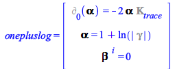
[advectiveonepluslog, generalizedharmonicslicing, geodesicslicing, harmoniccoordinates, harmonicslicing, kdriver, maximalslicing, onepluslog] (35)
 

To  see the condition equations behind these keywords in this first version of LapseAndShiftConditions, use 

> for condition in LapseAndShiftConditions() do _______________________________________; condition = LapseAndShiftConditions(condition) end do; 1
for condition in LapseAndShiftConditions() do _______________________________________; condition = LapseAndShiftConditions(condition) end do; 1

_______________________________________;
advectiveonepluslog = rtable(1 .. 2, [%LieDerivative[UnitNormalVector](Lapse) = `+`(`-`(`*`(2, `*`(%ExtrinsicCurvature[trace])))), `+`(%d_[0](Lapse), `-`(`*`(Shift[`~j`], `*`(%d_[j](Lapse))))) = `+`(`...
_______________________________________;
generalizedharmonicslicing = rtable(1 .. 2, [%d_[0](Lapse) = `+`(`-`(`*`(`^`(Lapse, 2), `*`(%f(Lapse), `*`(%ExtrinsicCurvature[trace]))))), Shift[`~i`] = 0], subtype = Vector[column]);
_______________________________________;
geodesicslicing = rtable(1 .. 2, [Lapse = 1, Shift[`~i`] = 0], subtype = Vector[column]);
_______________________________________;
harmoniccoordinates = rtable(1 .. 2, [`+`(%d_[0](Lapse), `-`(`*`(Shift[`~j`], `*`(%d_[j](Lapse))))) = `+`(`-`(`*`(`^`(Lapse, 2), `*`(%ExtrinsicCurvature[trace])))), `+`(%d_[0](Shift[`~i`]), `-`(`*`(Sh...
_______________________________________;
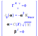
harmonicslicing = rtable(1 .. 3, [%d_[0](Lapse) = `+`(`-`(`*`(`^`(Lapse, 2), `*`(%ExtrinsicCurvature[trace])))), Lapse = `*`(%C(x, y, z, t), `*`(sqrt(%gamma3_[determinant]))), Shift[`~i`] = 0], subtyp...
_______________________________________;
kdriver = rtable(1 .. 3, [%d_[0](%ExtrinsicCurvature[trace]) = `*`(%c, `*`(%ExtrinsicCurvature[trace])), %d_[0](Lapse) = `+`(`-`(`*`(%epsilon, `*`(`+`(%d_[0](%ExtrinsicCurvature[trace]), `*`(%c, `*`(%...
_______________________________________;
maximalslicing = rtable(1 .. 2, [%ExtrinsicCurvature[trace] = 0, %d_[0](%ExtrinsicCurvature[trace]) = 0, D_[`~mu`](D_[mu](Lapse)) = `*`(Lapse, `*`(`+`(`*`(%ExtrinsicCurvature[mu, nu], `*`(%ExtrinsicCu...
_______________________________________;
Typesetting:-mrow(Typesetting:-mi( (36)


In the compact equations above, these condition equations for the Lapse and Shift include other tensors of the ThreePlusOne package, expressed in terms of their inert forms (displayed in grey) to allow for further manipulations. To retrieve these equations using these keywords, you can pass any them complete or, if you don't remember the exact spelling, just a portion of them suffices. For example, 

> LapseAndShiftConditions(generalized);

`*`(`* Partial match of  '`, `*`(generalized, `*`(`' against keyword '`, `*`(generalizedharmonicslicing, `*`(`' `)))));
Typesetting:-mfenced(Typesetting:-mrow(Typesetting:-mtable(Typesetting:-mtr(Typesetting:-mtd(Typesetting:-mrow(Typesetting:-mrow(Typesetting:-msub(Typesetting:-mi( (37)
 

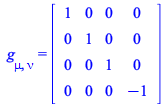
These conditions form a system of equations for the Lapse and Shift that, depending on the 4D metric set, may be solvable in exact form. For example, the metric set at this point is the default metric when Physics loads 

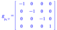
> g_[];
 

Typesetting:-mrow(Typesetting:-msub(Typesetting:-mi( (38)
 

and for this metric two exact solutions for the Lapse and Shift are 

> LapseAndShiftConditions(generalized, output = solution);

`*`(`* Partial match of  '`, `*`(generalized, `*`(`' against keyword '`, `*`(generalizedharmonicslicing, `*`(`' `)))));
{Physics:-ThreePlusOne:-Lapse = _F1(x, y, z), Physics:-ThreePlusOne:-Shift[`~1`] = 0, Physics:-ThreePlusOne:-Shift[`~2`] = 0, Physics:-ThreePlusOne:-Shift[`~3`] = 0}, {Physics:-ThreePlusOne:-Lapse = R... (39)
 

where the RootOf in the second set implies on 

> DEtools[remove_RootOf](alpha = RootOf(`+`(f(_Z), 1)));
 

`+`(f(Physics:-ThreePlusOne:-Lapse), 1) = 0 (40)
 

These results can be obtained step by step manipulating the equations (37) themselves, in which case it is more convenient to have them evaluated first. For that purpose use the option evaluate, and set the Lapse and Shift to arbitrary so that the ExtrinsicCurvature (or any other tensor of ThreePlusOne) is not prematurely evaluated in terms of the Minkowski metric (38) (comments about this further below) 

> Setup(lapse = arbitrary);

`*`(`* Partial match of  '`, `*`(lapse, `*`(`' against keyword '`, `*`(lapseandshift, `*`(`' `)))));
_______________________________________________________;
[lapseandshift = arbitrary] (41)
 

Now, instead of Kappa[trace]; = 0 we have the trace expressed in terms of arbitrary Lapse and Shift 

> ExtrinsicCurvature[trace];
 

Typesetting:-mprintslash([`+`(`-`(`/`(`*`(`+`(`*`(Physics:-ThreePlusOne:-Shift[`~1`], `*`(diff(Physics:-ThreePlusOne:-Lapse, x), `*`(`^`(Physics:-ThreePlusOne:-Lapse, 2)))), `*`(Physics:-ThreePlusOne:... (42)
 

and so, recomputing the equations LapseAndShiftConditions(generalized); using the evaluate option, we have 

> EQ := LapseAndShiftConditions(generalizedharmonicslicing, eval);

`*`(`* Partial match of  '`, `*`(eval, `*`(`' against keyword '`, `*`(evaluate, `*`(`' `)))));
Typesetting:-mfenced(Typesetting:-mrow(Typesetting:-mtable(Typesetting:-mtr(Typesetting:-mtd(Typesetting:-mrow(Typesetting:-mrow(Typesetting:-mi( (43)


Substitute the equations for the Shift, , into the equations for the Lapse alpha;  

> convert(EQ[2], setofequations);
 

{Physics:-ThreePlusOne:-Shift[`~1`] = 0, Physics:-ThreePlusOne:-Shift[`~2`] = 0, Physics:-ThreePlusOne:-Shift[`~3`] = 0} (44)
 

> subs({Physics:-ThreePlusOne:-Shift[`~1`] = 0, Physics:-ThreePlusOne:-Shift[`~2`] = 0, Physics:-ThreePlusOne:-Shift[`~3`] = 0}, EQ[1]);
 

Typesetting:-mprintslash([diff(Physics:-ThreePlusOne:-Lapse, t) = `+`(`-`(`*`(diff(Physics:-ThreePlusOne:-Lapse, t), `*`(f(Physics:-ThreePlusOne:-Lapse)))))], [Physics:-diff(Physics:-ThreePlusOne:-Lap... (45)
 

It is now possible to see that this system has two solutions: either f(alpha) = -1; (the second solution in (39), resulting in (40)) or the Lapse alpha; does not depend on t (the first solution in (39)). 


To understand the need, in (41), to set the
lapseandshift to arbitrary, check what happens with the default value Setup(lapse = standard);  

> Setup(lapse = standard);

`*`(`* Partial match of  '`, `*`(lapse, `*`(`' against keyword '`, `*`(lapseandshift, `*`(`' `)))));
_______________________________________________________;
[lapseandshift = standard] (46)
 

Trying to reproduce the computation above, the first step works 

> LapseAndShiftConditions(generalizedharmonicslicing, eval);
 

`*`(`* Partial match of  '`, `*`(eval, `*`(`' against keyword '`, `*`(evaluate, `*`(`' `)))));
Typesetting:-mfenced(Typesetting:-mrow(Typesetting:-mtable(Typesetting:-mtr(Typesetting:-mtd(Typesetting:-mrow(Typesetting:-mrow(Typesetting:-mi( (47)
 

but because of Setup(lapse = standard); , in the next step the derivative of the Lapse is computed rewriting the Lapse in terms of the Minkowski metric (38), for which the Lapse is actually equal to 1 

> Lapse(definition);
 

Typesetting:-mprintslash([Physics:-ThreePlusOne:-Lapse = `/`(1, `*`(sqrt(`+`(`-`(`*`(Physics:-D_[mu](t, [X]), `*`(Physics:-D_[`~mu`](t, [X]))))))))], [Physics:-ThreePlusOne:-Lapse = `/`(1, `*`(sqrt(`+... (48)
 

> SumOverRepeatedIndices(Physics:-ThreePlusOne:-Lapse = `/`(1, `*`(sqrt(`+`(`-`(`*`(Physics:-D_[mu](t, [X]), `*`(Physics:-D_[`~mu`](t, [X])))))))));
 

Physics:-ThreePlusOne:-Lapse = 1 (49)
 

and so, the step that results in (45), here results in nothing 

> subs({Physics:-ThreePlusOne:-Shift[`~1`] = 0, Physics:-ThreePlusOne:-Shift[`~2`] = 0, Physics:-ThreePlusOne:-Shift[`~3`] = 0}, EQ[1]);

0 = 0 (50)
 

The key observation is understanding what is defined (expressed) in terms of what. Given a 4D metric g[mu, nu]; , when Setup(lapseandshift = standard); the Lapse and Shift are defined in terms of the components g[0, mu]; . That is why in (49) we have alpha = 1; . On the other hand, when Setup(lapseandshift = arbitrary); the Lapse and Shift are not expressed in terms of the metric, they remain arbitrary, allowing for solving the condition equations in order to then express the components g[0, mu]; in terms of the Lapse and Shift. 

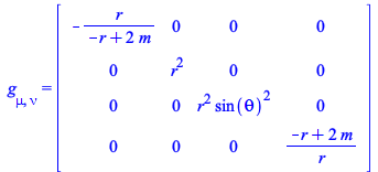
An example where the conditions can be solved exactly and the spacetime is curved: set the Schwarzschild metric in spherical coordinates 

> g_[sc];

_______________________________________________________;
`*`(`Systems of spacetime coordinates are:`, `*`({X = (r, theta, phi, t)}));
`*`(`Default differentiation variables for d_, D_ and dAlembertian are:`, `*`({X = (r, theta, phi, t)}));
`*`(`The Schwarzschild metric in coordinates `, `*`([r, theta, phi, t]));
`Parameters: `[m];
_______________________________________________________;
Typesetting:-mrow(Typesetting:-msub(Typesetting:-mi( (51)
 

Consider the harmonicslicing conditions 

> LapseAndShiftConditions(harmonicslicing);
 

Typesetting:-mfenced(Typesetting:-mrow(Typesetting:-mtable(Typesetting:-mtr(Typesetting:-mtd(Typesetting:-mrow(Typesetting:-msub(Typesetting:-mi( (52)
 

Note that in spite of having Setup(lapseandshift = standard); , in the internal intermediate computations of LapseAndShiftConditions Setup(lapseandshift = arbitrary); is used, so the problem can be formulated and tackled in the right way, resulting in the right conditions equations when using the option evaluate, allowing to compute a solution 

> LapseAndShiftConditions(harmonicslicing, evaluate);
 

Typesetting:-mfenced(Typesetting:-mrow(Typesetting:-mtable(Typesetting:-mtr(Typesetting:-mtd(Typesetting:-mrow(Typesetting:-mn(
(53)
 

> LapseAndShiftConditions(harmonicslicing, output = solution);
 

{Physics:-ThreePlusOne:-Lapse = `+`(`-`(`*`(`^`(sin(theta), `/`(1, 2)), `*`(`^`(_F1(r, theta, phi), `/`(1, 2)), `*`(r))))), m = m, Physics:-ThreePlusOne:-Shift[`~1`] = 0, Physics:-ThreePlusOne:-Shift[...
(54)

References 

  • [1] Alcubierre, M., Introduction to 3+1 Numerical Relativity, International Series of Monographs on Physics 140, Oxford University Press, 2008.

  • [2] Baumgarte, T.W., Shapiro, S.L., Numerical Relativity, Solving Einstein's Equations on a Computer, Cambridge University Press, 2010.


The new explore option of TensorArray

TensorArray is one of the most frequently used commands to see the components of tensors or tensorial expressions. The functionality is extremely useful and simple when the tensorial expression has at most 2 free indices, but things are not so simple when that number is 3 or larger. For this purpose, in Maple 2020 TensorArray has a new explore option, that allows for a quick and simple exploration of the components of tensorial expressions with an arbitrarily large number of indices. 

> with(Physics); -1
 

Although the new explore option is useful in general, the typical situation is that of tensorial expressions in curved spaces, so for illustration set the metric to something non-flat 

> ds2 := `+`(`-`(`*`(`^`(dt, 2))), `/`(`*`(`^`(a(t), 2), `*`(`^`(dr, 2))), `*`(`+`(`-`(`*`(k, `*`(`^`(r, 2)))), 1))), `*`(`^`(a(t), 2), `*`(`^`(r, 2), `*`(`^`(`dθ`, 2)))), `*`(`^`(a(t), 2), `*`(`^...
 

> Setup(coordinates = spherical, metric = ds2);


`*`(`Default differentiation variables for d_, D_ and dAlembertian are:`, `*`({X = (r, theta, phi, t)}));
`*`(`Systems of spacetime coordinates are:`, `*`({X = (r, theta, phi, t)}));
_______________________________________________________;
[coordinatesystems = {X}, metric = {(1, 1) = `/`(`*`(`^`(a(t), 2)), `*`(`+`(`-`(`*`(k, `*`(`^`(r, 2)))), 1))), (2, 2) = `*`(`^`(a(t), 2), `*`(`^`(r, 2))), (3, 3) = `*`(`^`(a(t), 2), `*`(`^`(r, 2), `*`... (55)
 

Define now two tensors 

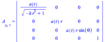
> A[mu, nu] = Matrix(4, {(1, 1) = `/`(`*`(a(t)), `*`(sqrt(`+`(`-`(`*`(k, `*`(`^`(r, 2)))), 1)))), (2, 2) = `*`(a(t), `*`(r)), (3, 3) = `*`(a(t), `*`(r, `*`(sin(theta)))), (4, 4) = 1});
 

Typesetting:-mrow(Typesetting:-msub(Typesetting:-mi( (56)
 

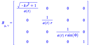
> B[mu, nu] = Matrix(4, {(1, 1) = `/`(`*`(sqrt(`+`(`-`(`*`(k, `*`(`^`(r, 2)))), 1))), `*`(a(t))), (2, 2) = `/`(1, `*`(a(t), `*`(r))), (3, 3) = `/`(1, `*`(a(t), `*`(r, `*`(sin(theta))))), (4, 4) = 1});
 

Typesetting:-mrow(Typesetting:-msub(Typesetting:-mi( (57)
 

>

;

`Defined objects with tensor properties`;
Typesetting:-mprintslash([[A[mu, nu], B[mu, nu], Physics:-D_[mu], Physics:-Dgamma[mu], Physics:-Psigma[mu], Physics:-Ricci[mu, nu], Physics:-Riemann[mu, nu, alpha, beta], Physics:-Weyl[mu, nu, alpha, ... (58)
 

Consider now the tensorial expression 

> `*`(A[nu, alpha], `*`(B[sigma, beta], `*`(Christoffel[nu, sigma, mu])));
 

`*`(B[beta, sigma], `*`(A[alpha, nu], `*`(Physics:-Christoffel[`~nu`, mu, `~sigma`]))) (59)

This expression has 3 free indices 

> Check(`*`(B[beta, sigma], `*`(A[alpha, nu], `*`(Physics:-Christoffel[`~nu`, mu, `~sigma`]))), free);

`*`(`The free indices are: `, `*`({`...`}));
{alpha, beta, mu} (60)
 

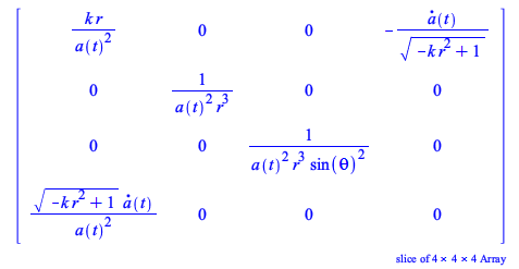
Passing this expression to TensorArray does not allow for a simple visualization because it only shows a slice of the 3-dimensional array of components 

> TensorArray(`*`(B[beta, sigma], `*`(A[alpha, nu], `*`(Physics:-Christoffel[`~nu`, mu, `~sigma`]))));
 

Typesetting:-msub(Typesetting:-mi( (61)
 

Moreover, there is the issue about which indices are being shown, in what order, and what is the value of the index not being shown. The interpretation of the matrix of components above is thus not straightforward.  

The new explore option compacts all the interactive information above ((59), (60), (61)) in one go and resolves the interpretation issues on the indices shown and not shown: 

> TensorArray(`*`(B[beta, sigma], `*`(A[alpha, nu], `*`(Physics:-Christoffel[`~nu`, mu, `~sigma`]))), explore);
 

(62)
 

`Index 1`


In this output we see: 

  • In the title, the tensorial expression being explored and an indication of its free indices, as well as the ordering used to produce the display (note that, for a tensorial expression, that ordering is not determined by the expression).

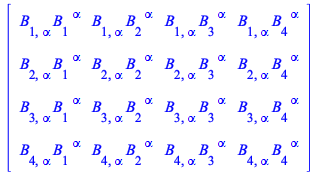
  • Which index is being explored: , making clear what is being displayed: the 2x2 slice for beta; and mu; (always the last two indices in the ordering list) when you take alpha = 1; .

  • You can move the slider 'Value of Index 1' to set the value of alpha; without having to recompute anything, and in that way see the different 2x2 slices for beta; and mu; .

  • You can actually choose which of the 3 indices will be 'Index 1' by clicking in the box surrounding alpha; , and in that way select the (remaining) indices that conform the 2x2 slice of components being shown (the ordering of indices in the 2x2 slice shown is always the one in the ordering list after you remove Index 1).

When the number of free indices is larger, being able to explore is even more significant. For example, for the product of the three non-contracted Ricci tensors `*`(R[alpha, rho], `*`(R[beta, nu], `*`(R[mu, sigma])));  

> TensorArray(`*`(Ricci[alpha, rho], `*`(Ricci[beta, nu], `*`(Ricci[mu, sigma]))), explore);
 

`*`(R[alpha, rho], `*`(R[beta, nu], `*`(R[mu, sigma], `*`(`      `(`ordering of free indices` = [alpha, beta, mu, nu, rho, sigma]))))); (63)
 

`Index 1` 

`Index 2` 

`Index 3` 

`Index 4` 

Embedded component 

Embedded component 

Embedded component 

Embedded component 


Embedded component 

`Value of Index 1` 

Embedded component 

1 

`Value of Index 2` 

Embedded component 

1 

`Value of Index 3` 

Embedded component 

1 

`Value of Index 4` 

Embedded component 

1 

The ability to specify the ordering of the free indices is relevant in general, but more specifically in the case of tensorial expressions like this one: although you can specify which indices are assuming values (and in that way chose their relative ordering) the information on the ordering of the indices of the 2x2 slice, being displayed in the title, may or may not be the one you want, and can only be adjusted with the option freeindices = [...]: the 2x2 slice always corresponds to the two indices of the ordering list that remain after you remove all of Index 1 to Index 4 (by default, they are the last two). So to change that use the option freeindices of TensorArray. 

Differentiating the spacetime metric, the tetrad, and their determinants, with respect to each other 

Maple 2020's Physics comes with several improvements in the underlying routines for differentiating tensorial expressions with respect to the spacetime metric, a relevant operation when computing field equations. The improvements also include differentiation of the tetrad `𝔢`[a, mu]; or with respect to it, of the determinant of the metric and the tetrad, and related manipulations with inert versions of these tensors. 

In what follows, the new differentiation formulas implemented in Maple 2020 are introduced, then the new manipulation capabilities are used to demonstrate them, finally these formulas are used in two examples: verifying a scalar identity and computing the energy-momentum tensor for the Proca Lagrangian density.
 

Differentiating the spacetime metricg[mu, nu]; with respect to itself

For illustration purposes set up the general case, that of an arbitrary metric 

> restart; 1; with(Physics); -1; with(Tetrads); -1; Setup(coordinates = X); -1; g_[arbitrary]; 1

_______________________________________________________;
`*`(`Setting `, `*`(lowercaselatin_ah, `*`(` letters to represent `, `*`(tetrad, `*`(` indices`)))));
`*`(`Defined as tetrad tensors `(`see ?Physics,tetrads`), `*`(`^`(`, `, 4), `*`(`𝔢`[a, mu], `*`(eta[a, b], `*`(gamma[a, b, c], `*`(lambda[a, b, c]))))));
`*`(`Defined as spacetime tensors representing the NP null vectors of the tetrad formalism `(`see ?Physics,tetrads`), `*`(`^`(`, `, 4), `*`(l[mu], `*`(n[mu], `*`(m[mu], `*`(conjugate(m[mu])))))));
_______________________________________________________;
`*`(`Default differentiation variables for d_, D_ and dAlembertian are:`, `*`({X = (x1, x2, x3, x4)}));
`*`(`Systems of spacetime coordinates are:`, `*`({X = (x1, x2, x3, x4)}));
_______________________________________________________;
Typesetting:-mrow(Typesetting:-msub(Typesetting:-mi( (64)
 

As it happens with any tensor, the derivative of the metric with respect to itself has an obvious result when the indices of the derivand and the differentiation metric have the same character (covariant or contravariant): 

> (%diff = diff)(g_[mu, nu], g_[alpha, beta]);
 

Typesetting:-mrow(Typesetting:-mrow(Typesetting:-mi( (65)
 

If the character of the derivand and the differentiation variable are the opposite, the result is less obvious: 

> (%diff = diff)(g_[mu, nu], g_[`~alpha`, `~beta`]);
 

Typesetting:-mrow(Typesetting:-mrow(Typesetting:-mi( (66)
 

Demonstration 

To demonstrate it, consider the identity 

> `*`(g_[mu, nu], `*`(g_[`~nu`, `~xi`])) = g_[mu, `~xi`];
 

`*`(Physics:-g_[mu, nu], `*`(Physics:-g_[`~nu`, `~xi`])) = Physics:-g_[mu, `~xi`] (67)
 

> Simplify(`*`(Physics:-g_[mu, nu], `*`(Physics:-g_[`~nu`, `~xi`])) = Physics:-g_[mu, `~xi`]);
 

Physics:-g_[mu, `~xi`] = Physics:-g_[mu, `~xi`] (68)
 

Differentiate this identity with respect to g[`~alpha`, `~beta`];  

> %diff(`*`(Physics:-g_[mu, nu], `*`(Physics:-g_[`~nu`, `~xi`])) = Physics:-g_[mu, `~xi`], g[`~alpha`, `~beta`]);
 

Typesetting:-mrow(Typesetting:-mi( (69)
 

Among the new manipulations possible in Maple 2020, you can expand inert derivatives without having them computed, an operation frequently required when deriving formulas 

> expand(%diff(`*`(Physics:-g_[mu, nu], `*`(Physics:-g_[`~nu`, `~xi`])) = Physics:-g_[mu, `~xi`], Physics:-g_[`~alpha`, `~beta`]));
 

Typesetting:-mrow(Typesetting:-mrow(Typesetting:-mrow(Typesetting:-mrow(Typesetting:-mi( (70)
 

The element we are interested in is a factor of the first term; isolate it 

> isolate(`+`(`*`(%diff(Physics:-g_[mu, nu], Physics:-g_[`~alpha`, `~beta`]), `*`(Physics:-g_[`~nu`, `~xi`])), `*`(Physics:-g_[mu, nu], `*`(%diff(Physics:-g_[`~nu`, `~xi`], Physics:-g_[`~alpha`, `~beta`...
 

Typesetting:-mrow(Typesetting:-mrow(Typesetting:-mrow(Typesetting:-mi( (71)
 

To remove g[`~nu`, `~xi`]; , multiply both sides of the equation by g[xi, rho]; , and use the dot operator `.` in order to multiply and simplify the indices in one go 

> Typesetting:-delayDotProduct(`*`(%diff(Physics:-g_[mu, nu], Physics:-g_[`~alpha`, `~beta`]), `*`(Physics:-g_[`~nu`, `~xi`])) = `+`(%diff(Physics:-g_[mu, `~xi`], Physics:-g_[`~alpha`, `~beta`]), `-`(`*...
 

Typesetting:-mrow(Typesetting:-mrow(Typesetting:-mi( (72)
 

On the right-hand side, the first derivative, %diff(g_[mu, `~xi`], g_[`~alpha`, `~beta`]); , is equal to zero since the derivand is a constant. The second derivative, %diff(g_[`~nu`, `~xi`], g_[`~alpha`, `~beta`]); is the easy case (65), so we have 

> lhs(%diff(Physics:-g_[mu, rho], Physics:-g_[`~alpha`, `~beta`]) = `*`(`+`(%diff(Physics:-g_[mu, `~xi`], Physics:-g_[`~alpha`, `~beta`]), `-`(`*`(Physics:-g_[mu, nu], `*`(%diff(Physics:-g_[`~nu`, `~xi`...
 

Typesetting:-mrow(Typesetting:-mrow(Typesetting:-mi( (73)
 

Simplifying the contracted indices we arrive at the desired result (66) 

> Simplify(%diff(Physics:-g_[mu, rho], Physics:-g_[`~alpha`, `~beta`]) = `+`(`-`(`*`(Physics:-g_[mu, nu], `*`(Physics:-g_[alpha, `~nu`], `*`(Physics:-g_[beta, `~xi`], `*`(Physics:-g_[rho, xi])))))));
 

Typesetting:-mrow(Typesetting:-mrow(Typesetting:-mi( (74)


Differentiating the tetrad `𝔢`[`~a`, alpha]; with respect to itself 

First the easy case, where the covariant and contravariant characters of the tensorial derivand and differentiation variable are the same 

> (%diff = diff)(`𝔢`[`~a`, alpha], `𝔢`[`~c`, nu]);
 

Typesetting:-mrow(Typesetting:-mrow(Typesetting:-mi( (75)
 

from where 

> (%diff = diff)(`𝔢`[`~a`, alpha], `𝔢`[c, nu]);
 

Typesetting:-mrow(Typesetting:-mrow(Typesetting:-mi( (76)
 

Differentiating with respect to the inverse tetrad: 

> (%diff = diff)(`𝔢`[`~a`, alpha], `𝔢`[c, `~nu`]);
 

Typesetting:-mrow(Typesetting:-mrow(Typesetting:-mi( (77)
 

Demonstration 

Consider the identity satisfied by the tetrad by definition 

> `*`(`𝔢`[`~a`, alpha], `*`(`𝔢`[a, `~beta`])) = g_[alpha, `~beta`];
 

`*`(Physics:-Tetrads:-e_[`~a`, alpha], `*`(Physics:-Tetrads:-e_[a, `~beta`])) = Physics:-g_[alpha, `~beta`] (78)
 

> Simplify(`*`(Physics:-Tetrads:-e_[`~a`, alpha], `*`(Physics:-Tetrads:-e_[a, `~beta`])) = Physics:-g_[alpha, `~beta`]);
 

Physics:-g_[alpha, `~beta`] = Physics:-g_[alpha, `~beta`] (79)
 

Differentiate this identity with respect to `𝔢`[c, `~nu`];  

> %diff(`*`(Physics:-Tetrads:-e_[`~a`, alpha], `*`(Physics:-Tetrads:-e_[a, `~beta`])) = Physics:-g_[alpha, `~beta`], `𝔢`[c, `~nu`]);
 

Typesetting:-mrow(Typesetting:-mi( (80)
 

> expand(%);
 

Typesetting:-mrow(Typesetting:-mrow(Typesetting:-mrow(Typesetting:-mrow(Typesetting:-mi( (81)
 

The element we are interested in is a factor of the first term; isolate it 

> isolate(`+`(`*`(%diff(Physics:-Tetrads:-e_[`~a`, alpha], Physics:-Tetrads:-e_[c, `~nu`]), `*`(Physics:-Tetrads:-e_[a, `~beta`])), `*`(Physics:-Tetrads:-e_[`~a`, alpha], `*`(%diff(Physics:-Tetrads:-e_[...
 

Typesetting:-mrow(Typesetting:-mrow(Typesetting:-mrow(Typesetting:-mi( (82)
 

To remove `𝔢`[a, `~beta`]; , multiply both sides of the equation by `𝔢`[`~b`, beta]; , and use the dot operator `.` in order to multiply and simplify the indices in one go 

> Typesetting:-delayDotProduct(`*`(%diff(Physics:-Tetrads:-e_[`~a`, alpha], Physics:-Tetrads:-e_[c, `~nu`]), `*`(Physics:-Tetrads:-e_[a, `~beta`])) = `+`(%diff(Physics:-g_[alpha, `~beta`], Physics:-Tetr...
 

Typesetting:-mrow(Typesetting:-mrow(Typesetting:-mi( (83)
 

On the right-hand side, the first derivative is equal to zero since the derivand is a constant. The second derivative is the easy case of differentiation of a tensor with respect to itself and same character of its indices, so we have 

> lhs(%diff(Physics:-Tetrads:-e_[`~b`, alpha], Physics:-Tetrads:-e_[c, `~nu`]) = `*`(`+`(%diff(Physics:-g_[alpha, `~beta`], Physics:-Tetrads:-e_[c, `~nu`]), `-`(`*`(Physics:-Tetrads:-e_[`~a`, alpha], `*...
 

Typesetting:-mrow(Typesetting:-mrow(Typesetting:-mi( (84)
 

The desired result, (77), is obtained simplifying the contracted indices 

> Simplify(%diff(Physics:-Tetrads:-e_[`~b`, alpha], Physics:-Tetrads:-e_[c, `~nu`]) = `+`(`-`(`*`(Physics:-Tetrads:-e_[`~a`, alpha], `*`(Physics:-Tetrads:-eta_[a, `~c`], `*`(Physics:-g_[nu, `~beta`], `*...
 

Typesetting:-mrow(Typesetting:-mrow(Typesetting:-mi( (85)


Differentiating the spacetime metric g[alpha, beta]; with respect to the tetrad `𝔢`[a, nu];  

> (%diff = diff)(g[alpha, beta], `𝔢`[a, nu]);
 

Typesetting:-mrow(Typesetting:-mrow(Typesetting:-mi( (86)
 

Demonstration 

Depart from the definition `*`(`𝔢`[`~a`, alpha], `*`(`𝔢`[a, `~beta`])) = g_[alpha, `~beta`]; with both spacetime indices covariant 

> g_[alpha, beta] = `*`(e_[`~c`, alpha], `*`(e_[c, beta]));
 

Physics:-g_[alpha, beta] = `*`(Physics:-Tetrads:-e_[`~c`, alpha], `*`(Physics:-Tetrads:-e_[c, beta])) (87)
 

> %diff(Physics:-g_[alpha, beta] = `*`(Physics:-Tetrads:-e_[`~c`, alpha], `*`(Physics:-Tetrads:-e_[c, beta])), `𝔢`[a, nu]);
 

Typesetting:-mrow(Typesetting:-mi( (88)
 

> expand(%diff(Physics:-g_[alpha, beta] = `*`(Physics:-Tetrads:-e_[`~c`, alpha], `*`(Physics:-Tetrads:-e_[c, beta])), Physics:-Tetrads:-e_[a, nu]));
 

Typesetting:-mrow(Typesetting:-mrow(Typesetting:-mi( (89)
 

Results for the two derivatives on the right-hand side were already derived in the previous sections, so 

> lhs(%diff(Physics:-g_[alpha, beta], Physics:-Tetrads:-e_[a, nu]) = `+`(`*`(%diff(Physics:-Tetrads:-e_[`~c`, alpha], Physics:-Tetrads:-e_[a, nu]), `*`(Physics:-Tetrads:-e_[c, beta])), `*`(Physics:-Tetr...
 

Typesetting:-mrow(Typesetting:-mrow(Typesetting:-mi( (90)
 

> Simplify(%diff(Physics:-g_[alpha, beta], Physics:-Tetrads:-e_[a, nu]) = `+`(`*`(Physics:-Tetrads:-e_[c, beta], `*`(Physics:-Tetrads:-eta_[`~a`, `~c`], `*`(Physics:-g_[alpha, `~nu`]))), `*`(Physics:-Te...
 

Typesetting:-mrow(Typesetting:-mrow(Typesetting:-mi( (91)
 

Analogously, 

> (%diff = diff)(g[alpha, beta], `𝔢`[`~a`, nu]);
 

Typesetting:-mrow(Typesetting:-mrow(Typesetting:-mi( (92)
 

Differentiating with respect to the inverse tetrad changes a sign 

> (%diff = diff)(g[alpha, beta], `𝔢`[a, `~nu`]);
 

Typesetting:-mrow(Typesetting:-mrow(Typesetting:-mi( (93)
 

This result can be demostrated as done above for %diff(g_[alpha, beta], e_[a, nu]); , changing `𝔢`[a, nu]; by `𝔢`[a, `~nu`];  

Example: the vanishing of certain combinations of derivatives of a scalar 


For background on this example, see the Appendix in: J. Struckmeier, D. Vasak1, and J. Kirsch1, "Generic Theory of Geometrodynamics from Noether's theorem for the Diff(M) symmetry group" . Define two arbitrary 2-rank tensors and use them to define a scalar S 

> Define(A[alpha, beta], B[alpha, beta]);

`Defined objects with tensor properties`;
Typesetting:-mprintslash([[A[alpha, beta], B[alpha, beta], Physics:-D_[mu], Physics:-Dgamma[mu], Physics:-Psigma[mu], Physics:-Ricci[mu, nu], Physics:-Riemann[mu, nu, alpha, beta], Physics:-Weyl[mu, n... (94)
 

> S__1 := `+`(`*`(A[`~alpha`, `~beta`], `*`(g[alpha, beta])), `*`(B[xi, eta], `*`(g[`~xi`, `~eta`])));
 

Typesetting:-mprintslash([S__1 := `+`(`*`(A[`~alpha`, `~beta`], `*`(Physics:-g_[alpha, beta])), `*`(B[xi, eta], `*`(Physics:-g_[`~eta`, `~xi`])))], [`+`(`*`(A[`~alpha`, `~beta`], `*`(Physics:-g_[alpha... (95)
 

The following combination of derivatives is equal to 0; use delay evaluation quotes to see the expression echoed in the output, more readable with typesetting 

> '`+`(`*`(%diff(S__1, `𝔢`[f, `~nu`]), `*`(`𝔢`[f, `~mu`])), `*`(%diff(S__1, A[`~nu`, `~eta`]), `*`(A[`~mu`, `~eta`])), `*`(%diff(S__1, A[`~eta`, `~nu`]), `*`(A[eta, `~mu`])), `-`(`*`(%diff(S__1,...
 

Typesetting:-mrow(Typesetting:-mrow(Typesetting:-mrow(Typesetting:-mi( (96)
 

Unleash the delay evaluation quotes '' 

> `+`(Physics:-`*`(%diff(S__1, Physics:-Tetrads:-e_[f, `~nu`]), Physics:-Tetrads:-e_[f, `~mu`]), Physics:-`*`(%diff(S__1, A[`~nu`, `~eta`]), A[`~mu`, `~eta`]), Physics:-`*`(%diff(S__1, A[`~eta`, `~nu`])...
 

Typesetting:-mrow(Typesetting:-mrow(Typesetting:-mrow(Typesetting:-mrow(Typesetting:-mi(
(97)
 

Compute a value for (i.e., activate) the inert derivatives 

> value(`+`(`*`(%diff(`+`(`*`(A[`~alpha`, `~beta`], `*`(Physics:-g_[alpha, beta])), `*`(B[xi, eta], `*`(Physics:-g_[`~eta`, `~xi`]))), Physics:-Tetrads:-e_[f, `~nu`]), `*`(Physics:-Tetrads:-e_[f, `~mu`]...
 

`+`(`*`(`+`(`*`(A[`~alpha`, `~beta`], `*`(`+`(`-`(`*`(Physics:-Tetrads:-e_[`~f`, alpha], `*`(Physics:-g_[beta, nu]))), `-`(`*`(Physics:-Tetrads:-e_[`~f`, beta], `*`(Physics:-g_[alpha, nu])))))), `*`(B...
(98)
 

> Simplify(`+`(`*`(`+`(`*`(A[`~alpha`, `~beta`], `*`(`+`(`-`(`*`(Physics:-Tetrads:-e_[`~f`, alpha], `*`(Physics:-g_[beta, nu]))), `-`(`*`(Physics:-Tetrads:-e_[`~f`, beta], `*`(Physics:-g_[alpha, nu]))))...
 

0 = 0 (99)
 

An alternative formulation expressing the spacetime metric entering S in terms of tetrads  

> S__2 := `+`(`*`(`𝔢`[c, `~xi`], `*`(`𝔢`[d, `~eta`], `*`(B[xi, eta], `*`(eta[`~c`, `~d`])))), `*`(`𝔢`[`~a`, alpha], `*`(`𝔢`[`~b`, beta], `*`(A[`~alpha`, `~beta`], `*`(eta[a, b])))));
 

Typesetting:-mprintslash([S__2 := `+`(`*`(A[`~alpha`, `~beta`], `*`(Physics:-Tetrads:-e_[`~a`, alpha], `*`(Physics:-Tetrads:-e_[`~b`, beta], `*`(Physics:-Tetrads:-eta_[a, b])))), `*`(B[xi, eta], `*`(P... (100)
 

> subs(S__1 = S__2, `+`(Physics:-`*`(%diff(S__1, Physics:-Tetrads:-e_[f, `~nu`]), Physics:-Tetrads:-e_[f, `~mu`]), Physics:-`*`(%diff(S__1, A[`~nu`, `~eta`]), A[`~mu`, `~eta`]), Physics:-`*`(%diff(S__1,...
 

Typesetting:-mrow(Typesetting:-mrow(Typesetting:-mrow(Typesetting:-mrow(Typesetting:-mi(
(101)
 

> value(`+`(`*`(%diff(`+`(`*`(A[`~alpha`, `~beta`], `*`(Physics:-Tetrads:-e_[`~a`, alpha], `*`(Physics:-Tetrads:-e_[`~b`, beta], `*`(Physics:-Tetrads:-eta_[a, b])))), `*`(B[xi, eta], `*`(Physics:-Tetrad...
 

`+`(`*`(`+`(`-`(`*`(A[`~alpha`, `~beta`], `*`(Physics:-Tetrads:-e_[`~a`, alpha], `*`(Physics:-Tetrads:-e_[`~b`, nu], `*`(Physics:-Tetrads:-e_[`~f`, beta], `*`(Physics:-Tetrads:-eta_[a, b])))))), `-`(`...
(102)
 

> Simplify(`+`(`*`(`+`(`-`(`*`(A[`~alpha`, `~beta`], `*`(Physics:-Tetrads:-e_[`~a`, alpha], `*`(Physics:-Tetrads:-e_[`~b`, nu], `*`(Physics:-Tetrads:-e_[`~f`, beta], `*`(Physics:-Tetrads:-eta_[a, b]))))...
 

0 = 0 (103)
 

Differentiating the determinant of the metric with respect to the metric 

The following results are necessary when one works with relative tensors of some weight and in particular with tensor densities. This derivative is also relevant in general relativity when computing field equations.  

Given any 2-rank tensor (representable by a 2x2 matrix), the design in the Physics package is that its determinant is computed when you index the tensor with the keyword determinant. For example, for the arbitrary metric g_ set at this point, 

> g_[determinant];
 

`+`(`*`(`+`(`-`(`*`(_F8(X), `*`(_F10(X)))), `*`(`^`(_F9(X), 2))), `*`(`^`(_F2(X), 2))), `*`(`+`(`*`(`+`(`*`(2, `*`(_F6(X), `*`(_F10(X)))), `-`(`*`(2, `*`(_F7(X), `*`(_F9(X)))))), `*`(_F3(X))), `-`(`*`...
(104)
 

Depending on the formulation, however, to perform algebraic manipulations what is required is a representation of the determinant, not its computed value. For that purpose use the inert form 

> %g_[determinant];
 

Typesetting:-msub(Typesetting:-mi( (105)
 

that you can activate when desired using value .  

> value(%g_[determinant]);
 

`+`(`*`(`+`(`-`(`*`(_F8(X), `*`(_F10(X)))), `*`(`^`(_F9(X), 2))), `*`(`^`(_F2(X), 2))), `*`(`+`(`*`(`+`(`*`(2, `*`(_F6(X), `*`(_F10(X)))), `-`(`*`(2, `*`(_F7(X), `*`(_F9(X)))))), `*`(_F3(X))), `-`(`*`...
(106)
 

From the general rule for the derivative of the determinant of a matrix M with respect to one of its components, , taking M = g[mu, nu]; and `/`(1, `*`(M)) = g[`~mu`, `~nu`]; , the derivative of the determinant of the metric is proportional to itself, and this rule is understood in Maple 2020 when you use the inert representation %g_[determinant];  

> (%diff = diff)(%g_[determinant], g[mu, nu]);
 

Typesetting:-mrow(Typesetting:-mrow(Typesetting:-mi( (107)
 

The derivative with respect to the contravariant components follows from the above by taking into account that delta(`*`(g[`~mu`, `~nu`], `*`(g[mu, nu]))) = 0; , hence `*`(g[`~mu`, `~nu`], `*`(delta, `*`(g[mu, nu]))) = `+`(`-`(`*`(g[`~mu`, `~nu`], `*`(delta, `*`(g[mu, nu]))))); so that 

> (%diff = diff)(%g_[determinant], g[`~mu`, `~nu`]);
 

Typesetting:-mrow(Typesetting:-mrow(Typesetting:-mi( (108)
 

Analogously, the derivative of the determinant of the tetrad with respect to the tetrad is computed using the inert form %e_ to represent the determinant 

> (%diff = diff)(%e_[determinant], `𝔢`[a, nu]);
 

Typesetting:-mrow(Typesetting:-mrow(Typesetting:-mi( (109)
 

> (%diff = diff)(%e_[determinant], `𝔢`[a, `~nu`]);
 

Typesetting:-mrow(Typesetting:-mrow(Typesetting:-mi( (110)
 

> (%diff = diff)(%e_[determinant], `𝔢`[`~a`, nu]);
 

Typesetting:-mrow(Typesetting:-mrow(Typesetting:-mi( (111)
 

Consequently, 

> (%diff = diff)(sqrt(`+`(`-`(%g_[determinant]))), `𝔢`[`~a`, nu]);
 

Typesetting:-mrow(Typesetting:-mrow(Typesetting:-mi( (112)
 

Demonstration 

Demonstrations for all of (109), (110) or (111) can be done in one and the same way: depart from the identity (87) written in terms of the all covariant tetrad 

`*`(eta[`~a`, `~b`], `*`(`𝔢`[b, alpha], `*`(`𝔢`[a, beta]))) = g[alpha, beta];  

Taking the determinant of each side of this equation, defining `≡`(e_[determinant], det(`𝔢`[a, beta])); and recalling that the determinant of a product is equal to the product of the determinants, 

`*`(%eta_[determinant], `*`(`^`(%e_[determinant], 2))) = %g_[determinant];  

In the case of an orthonormal tetrad, %eta_[determinant] = -1; , while for a null tetrad, %eta_[determinant] = 1; . So in both cases we can rewrite this expression as 

`*`(`^`(e_[determinant], 2)) = `*`(eta_[determinant], `*`(g_[determinant]));  

From where, choosing the principal branch of the square root, 

> %e_[determinant] = sqrt(`*`(%eta_[determinant], `*`(%g_[determinant])));

%e_[determinant] = `*`(`^`(`*`(%eta_[determinant], `*`(%g_[determinant])), `/`(1, 2))) (113)


Note: in the case of a null tetrad, eta_[determinant] = 1; , and so `and`(`≡`(e_[determinant], det(`𝔢`[a, beta])) = det(`*`(eta[a, b], `*`(`𝔢`[`~b`, beta]))), det(`*`(eta[a, b], `*`(`𝔢`[`~b`, beta]))) = det(`𝔢`[`~a`, beta])); . On the other hand, in the (default) case of an orthonormal tetrad, eta[a, b]; is a Minkowski metric with eta_[determinant] = -1; , and so det(`𝔢`[a, beta]) = `+`(`-`(det(`𝔢`[`~a`, beta])));  


Differentiating %e_[determinant]; with respect to the tetrad 

> %diff(%e_[determinant] = `*`(`^`(`*`(%eta_[determinant], `*`(%g_[determinant])), `/`(1, 2))), `𝔢`[a, nu]);

Typesetting:-mrow(Typesetting:-mi( (114)

> expand(%diff(%e_[determinant] = `*`(`^`(`*`(%eta_[determinant], `*`(%g_[determinant])), `/`(1, 2))), Physics:-Tetrads:-e_[a, nu]));

Typesetting:-mrow(Typesetting:-mrow(Typesetting:-mi( (115)

Using the chain rule and the differentiation rules for %diff(%g_[determinant], %e_[a, nu]); derived in the previous sections we obtain 

> lhs(%diff(%e_[determinant], Physics:-Tetrads:-e_[a, nu]) = %diff(`*`(`^`(`*`(%eta_[determinant], `*`(%g_[determinant])), `/`(1, 2))), Physics:-Tetrads:-e_[a, nu])) = eval(rhs(%diff(%e_[determinant], P...
 

Typesetting:-mrow(Typesetting:-mrow(Typesetting:-mi( (116)
 

which in view of (113) can be written as %diff(%e_[determinant], e_[a, nu]) = `*`(`𝔢`[`~a`, `~nu`], `*`(%e_[determinant]));  

For (110), 

> subs(`𝔢`[a, nu] = `𝔢`[a, `~nu`], %diff(%e_[determinant], Physics:-Tetrads:-e_[a, nu]) = %diff(`*`(`^`(`*`(%eta_[determinant], `*`(%g_[determinant])), `/`(1, 2))), Physics:-Tetrads:-e_[a, nu]))...
 

Typesetting:-mrow(Typesetting:-mrow(Typesetting:-mi( (117)
 

> lhs(%diff(%e_[determinant], Physics:-Tetrads:-e_[a, `~nu`]) = %diff(`*`(`^`(`*`(%eta_[determinant], `*`(%g_[determinant])), `/`(1, 2))), Physics:-Tetrads:-e_[a, `~nu`])) = eval(rhs(%diff(%e_[determina...
 

Typesetting:-mrow(Typesetting:-mrow(Typesetting:-mi( (118)
 

Taking into account (113) this result can be written as %diff(%e_[determinant], e_[a, `~nu`]) = `+`(`-`(`*`(`𝔢`[`~a`, nu], `*`(%e_[determinant]))));  

Example: the components of the Energy-Momentum tensor for the Proca Lagrangian density

To express the Proca Lagrangian density, define the tensors entering the formulation

> Define(a[mu], T[mu, nu]);

`Defined objects with tensor properties`;
Typesetting:-mprintslash([[A[alpha, beta], B[alpha, beta], Physics:-D_[mu], Physics:-Dgamma[mu], Physics:-Psigma[mu], Physics:-Ricci[mu, nu], Physics:-Riemann[mu, nu, alpha, beta], T[mu, nu], Physics:... (119)

> Define(f[mu, nu], antisymmetric);


`Defined objects with tensor properties`;
Typesetting:-mprintslash([[A[alpha, beta], B[alpha, beta], Physics:-D_[mu], Physics:-Dgamma[mu], Physics:-Psigma[mu], Physics:-Ricci[mu, nu], Physics:-Riemann[mu, nu, alpha, beta], T[mu, nu], Physics:... (120)
 

The Lagrangian: 

> L := `*`(`+`(`-`(`*`(`/`(1, 4), `*`(f[alpha, beta], `*`(f[xi, eta], `*`(g[`~alpha`, `~xi`], `*`(g[`~beta`, `~eta`])))))), `*`(`/`(1, 2), `*`(`^`(m, 2), `*`(a[alpha], `*`(a[xi], `*`(g[`~alpha`, `~xi`])...
 

Typesetting:-mprintslash([L := `*`(`+`(`-`(`*`(`/`(1, 4), `*`(f[alpha, beta], `*`(f[xi, eta], `*`(Physics:-g_[`~alpha`, `~xi`], `*`(Physics:-g_[`~beta`, `~eta`])))))), `*`(`/`(1, 2), `*`(`^`(m, 2), `*... (121)
 

By definition, the contravariant components of the energy momentum tensor are given by 

> T[`~nu`, `~mu`] = `+`(`-`(`/`(`*`(2, `*`(%diff(%L, g[nu, mu]))), `*`(sqrt(`+`(`-`(%g_[determinant])))))));
 

Typesetting:-mrow(Typesetting:-msub(Typesetting:-mi( (122)
 

Instead of using value on the whole expression, which would result in the computation of %g_[determinant]; , selectively activate %diff and %L 

> eval(T[`~nu`, `~mu`] = `+`(`-`(`/`(`*`(2, `*`(%diff(%L, Physics:-g_[mu, nu]))), `*`(`^`(`+`(`-`(%g_[determinant])), `/`(1, 2)))))), [%L = L, %diff = diff]);
 

T[`~nu`, `~mu`] = `+`(`-`(`/`(`*`(2, `*`(`+`(`-`(`/`(`*`(`/`(1, 2), `*`(`+`(`-`(`*`(`/`(1, 4), `*`(f[alpha, beta], `*`(f[xi, eta], `*`(Physics:-g_[`~alpha`, `~xi`], `*`(Physics:-g_[`~beta`, `~eta`])))...
(123)
 

Simplifying the contracted tensor indices we get the expected result 

> Simplify(T[`~nu`, `~mu`] = `+`(`-`(`/`(`*`(2, `*`(`+`(`-`(`/`(`*`(`/`(1, 2), `*`(`+`(`-`(`*`(`/`(1, 4), `*`(f[alpha, beta], `*`(f[xi, eta], `*`(Physics:-g_[`~alpha`, `~xi`], `*`(Physics:-g_[`~beta`, `...
 

T[`~nu`, `~mu`] = `+`(`*`(`/`(1, 4), `*`(Physics:-g_[`~mu`, `~nu`], `*`(`+`(`-`(`*`(2, `*`(`^`(m, 2), `*`(a[beta], `*`(a[`~beta`]))))), `*`(f[beta, xi], `*`(f[`~beta`, `~xi`])))))), `*`(`^`(m, 2), `*`... (124)
 

Simplifying spinor, su2, su3 and gauge indices 

In previous releases, the Simplify command, for simplifying among other things tensorial expressions, only handled spacetime, space and tetrad indices. In Maple 2020, Simplify also handle spinor, su2, su3 and/or gauge indices taking into account Einstein's sum rule for repeated indices and the possible existence of tensor symmetries. As in previous releases, the tensors are defined as such using Define, and the letters used to represent different kinds of indices are set using Setup, for example:  

Unlike the case of spacetime indices, that can refer to a curved or Minkowski space where the metric is not Euclidean, the metric for spinor, su2, su3 and gauge indices is always Euclidean and represented by KroneckerDelta indexed with indices of the corresponding type. In connection with this development, the dimension of the spaces represented by these indices is automatically set according to: 

  • Spinor indices (spinorindices keyword of Setup ) are assumed to have the dimension of the Dirac matrices. These are the indices to use when making explicit the matrix indices of the Dirac matrices , also defined as a spacetime vector `^`(gamma, mu); . The matrix indices are entered as a second indexation, Dgamma[mu][i, j]; . Spinor indices can also be used to index Dirac spinors, anticommutative objects, relevant in quantum field theory (see Maple 2020 developments for computing the Scattering matrix and Feynman Diagrams in coordinates and momentum representation). In a 4-dimensional spacetime, these indices run from 1 to 4 (not from 0 to 3). Note that, in general, Dirac matrices are `*`(`^`(N, 2), `*`(x)); where N = `^`(2, floor(`+`(`*`(`/`(1, 2), `*`(spacetime, `*`(dimension)))))); , so only when `*`(spacetime, `*`(dimension)) = 4; is that the spacetime and spinor dimensions are equal.

  • The SU(2) indices (su2indices keyword of Setup ) run from 1 to 3, the dimension of the group (number of generators of SU(2)), and are appropriate as the vector index for redefining Pauli matrices , that are defined as a spacetime vector `σ__μ`; when Physics is loaded .

  • The SU(2) matrix indices (new su2matrixindices keyword of Setup ) run from 1 to 2, the dimension of the 2x2 matrix elements of SU(2) in the fundamental representation, and are appropriate as the matrix indices for each of the `^`(sigma, mu); Pauli matrices . These indices are entered as a second indexation, e.g. Psigma[mu][i, j]; .

  • The SU(3) indices (su3indices keyword of Setup) run from 1 to 8, the dimension of the group (number of generators of SU(3)), and are appropriate as the vector index for the Gell-Mann matrices , implemented in the StandardModel subpackage as an 8-dimensional vector G__a; .

  • The SU(3) matrix indices (new su3matrixindices keyword of Setup) run from 1 to 3, the dimension of the 3x3 matrix elements of SU(3) in the fundamental representation, and are appropriate as the matrix indices for each of the . These indices are entered as a second indexation, e.g. Glambda[a][i, j]; .

  • The Setup command accepts one more kind of indices: gaugeindices, that can be used to represent more generic objects in an Euclidean space of undefined dimension.


Examples 

> restart; 1; with(Physics); -1

Set spinor, su2 and su3 indices, also an anticommutative prefix to represent a Dirac spinor 

> Setup(anticommutativeprefix = psi, spinorindices = lowercaselatin_is, su2indices = lowercaselatin_ah, su2matrixindices = uppercaselatin);
 

[anticommutativeprefix = {psi}, spinorindices = lowercaselatin_is, su2indices = lowercaselatin_ah, su2matrixindices = uppercaselatin] (125)
 

To work with a Dirac spinor using tensor notation, define it first as a tensor 

> Define(psi[j]);

`Defined objects with tensor properties`;
{Physics:-Dgamma[mu], Physics:-Psigma[mu], Physics:-d_[mu], Physics:-g_[mu, nu], psi[j], Physics:-LeviCivita[alpha, beta, mu, nu]} (126)
 

In view of the anticommutative character of psi[j]; , the following two expressions are zero 

> `*`(psi[j], `*`(psi[k], `*`(KroneckerDelta[j, k])));
 

Typesetting:-mprintslash([`*`(Physics:-KroneckerDelta[j, k], `*`(Physics:-`*`(psi[j], psi[k])))], [`*`(Physics:-KroneckerDelta[j, k], `*`(Physics:-`*`(psi[j], psi[k])))]) (127)
 

> Simplify(`*`(Physics:-KroneckerDelta[j, k], `*`(Physics:-`*`(psi[j], psi[k]))));
 

0 (128)
 

> `*`(psi[j], `*`(psi[k], `*`(LeviCivita[j, m, n], `*`(LeviCivita[k, m, n]))));
 

Typesetting:-mprintslash([`*`(Physics:-LeviCivita[j, m, n], `*`(Physics:-LeviCivita[k, m, n], `*`(Physics:-`*`(psi[j], psi[k]))))], [`*`(Physics:-LeviCivita[j, m, n], `*`(Physics:-LeviCivita[k, m, n],... (129)
 

> Simplify(`*`(Physics:-LeviCivita[j, m, n], `*`(Physics:-LeviCivita[k, m, n], `*`(Physics:-`*`(psi[j], psi[k])))));
 

0 (130)
 

To understand the result above, split the product into two factors, separating the part that contains LeviCivita tensors 

> [selectremove(has, `*`(Physics:-LeviCivita[j, m, n], `*`(Physics:-LeviCivita[k, m, n], `*`(Physics:-`*`(psi[j], psi[k])))), LeviCivita)];
 

Typesetting:-mprintslash([[`*`(Physics:-LeviCivita[j, m, n], `*`(Physics:-LeviCivita[k, m, n])), Physics:-`*`(psi[j], psi[k])]], [[`*`(Physics:-LeviCivita[j, m, n], `*`(Physics:-LeviCivita[k, m, n])),... (131)
 

Simplify each part 

> map(Simplify, [`*`(Physics:-LeviCivita[j, m, n], `*`(Physics:-LeviCivita[k, m, n])), Physics:-`*`(psi[j], psi[k])]);
 

Typesetting:-mprintslash([[`+`(`*`(2, `*`(Physics:-KroneckerDelta[j, k]))), Physics:-`*`(psi[j], psi[k])]], [[`+`(`*`(2, `*`(Physics:-KroneckerDelta[j, k]))), Physics:-`*`(psi[j], psi[k])]]) (132)
 

From Simplify(`*`(Physics:-KroneckerDelta[j, k], `*`(Physics:-`*`(psi[j], psi[k])))); ,  `*`(epsilon[j, m, n], `*`(epsilon[k, m, n], `*`(psi[j], `*`(psi[k])))) = 0;  

Related to the ability to simplify and manipulate su2 and su3 indices, the Library:-PerformMatrixOperations command got further developed. For example, consider the fully contracted product of Pauli matrices, both regarding their spacetime index mu; and their su2matrix indices A, B;  

> `*`(sigma[nu][A, B], `*`(sigma[`~nu`][B, A]));
 

Typesetting:-mprintslash([Physics:-`*`(Physics:-Psigma[nu][A, B], Physics:-Psigma[`~nu`][B, A])], [Physics:-`*`(Physics:-Psigma[nu][A, B], Physics:-Psigma[`~nu`][B, A])]) (133)
 

> Library:-PerformMatrixOperations(Physics:-`*`(Physics:-Psigma[nu][A, B], Physics:-Psigma[`~nu`][B, A]));
 

-4 (134)
 

As a more involved case example, consider for instance a Yang-Mills theory with a massless field B[mu, a]; where a is a SU2 index (see eq.(12) of sec. 19.4 of ref.[1]). The interaction Lagrangian can be entered as follows: 

> Setup(coordinates = cartesian, massless = B, op = B);

`*`(`* Partial match of  '`, `*`(massless, `*`(`' against keyword '`, `*`(masslessfields, `*`(`' `)))));
`*`(`* Partial match of  '`, `*`(op, `*`(`' against keyword '`, `*`(quantumoperators, `*`(`' `)))));
`*`(`Default differentiation variables for d_, D_ and dAlembertian are:`, `*`({X = (x, y, z, t)}));
`*`(`Systems of spacetime coordinates are:`, `*`({X = (x, y, z, t)}));
_______________________________________________________;
[coordinatesystems = {X}, masslessfields = {B}, quantumoperators = {B}] (135)
 

> Define(B[mu, a]);

`Defined objects with tensor properties`;
Typesetting:-mprintslash([[B[mu, a], Physics:-Dgamma[mu], Physics:-Psigma[mu], Physics:-d_[mu], Physics:-g_[mu, nu], psi[j], Physics:-LeviCivita[alpha, beta, mu, nu], X[mu]]], [{B[mu, a], Physics:-Dga... (136)


Use a compact display to avoid redundant display of functionality 

> CompactDisplay(B(X));
 

`*`(` B`(X), `*`(`will now be displayed as`, `*`(B))) (137)
 

> F__B[mu, nu, a] := `+`(d_[mu](B[nu, a](X)), `-`(d_[nu](B[mu, a](X))));
 

Typesetting:-mrow(Typesetting:-mrow(Typesetting:-msub(Typesetting:-mi( (138)
 

The Lagrangian: 

> L := `+`(`*`(`/`(1, 2), `*`(q, `*`(LeviCivita[a, b, c], `*`(F__B[mu, nu, a], `*`(B[mu, b](X), `*`(B[nu, c](X))))))), `*`(`/`(1, 4), `*`(`^`(q, 2), `*`(LeviCivita[a, b, c], `*`(LeviCivita[a, e, f], `*`...
L := `+`(`*`(`/`(1, 2), `*`(q, `*`(LeviCivita[a, b, c], `*`(F__B[mu, nu, a], `*`(B[mu, b](X), `*`(B[nu, c](X))))))), `*`(`/`(1, 4), `*`(`^`(q, 2), `*`(LeviCivita[a, b, c], `*`(LeviCivita[a, e, f], `*`...
 

Typesetting:-mrow(Typesetting:-mrow(Typesetting:-mfrac(Typesetting:-mn( (139)
 

The transition probability density at tree-level for a process with two incoming and two outgoing B particles, that is %eval(`#mfenced(mrow(mo(, where S is the Scattering matrix, is given by 

> FeynmanDiagrams(L, incomingparticles = [B, B], outgoingparticles = [B, B], numberofloops = 0);
 

Typesetting:-mprintslash([`+`(`/`(`*`(`*`(`/`(1, 8), `*`(I)), `*`(Physics:-FeynmanDiagrams:-PolarizationVector[B][alpha, d](P__1_), `*`(Physics:-FeynmanDiagrams:-PolarizationVector[B][beta, g](P__2_),...
(140)
 

Due to the use of size simplification, this expression is of computational length ~4000 and has only 4 terms, although each of them nested several times 

> number_of_factors = nops(`+`(`/`(`*`(`*`(`/`(1, 8), `*`(I)), `*`(Physics:-FeynmanDiagrams:-PolarizationVector[B][alpha, d](P__1_), `*`(Physics:-FeynmanDiagrams:-PolarizationVector[B][beta, g](P__2_), ...
 

number_of_factors = 4, computational_length = 4036 (141)
 

> codegen:-cost(`+`(`/`(`*`(`*`(`/`(1, 8), `*`(I)), `*`(Physics:-FeynmanDiagrams:-PolarizationVector[B][alpha, d](P__1_), `*`(Physics:-FeynmanDiagrams:-PolarizationVector[B][beta, g](P__2_), `*`(conjuga...
 

`+`(`*`(68, `*`(additions)), `*`(125, `*`(multiplications)), `*`(124, `*`(subscripts)), `*`(7, `*`(divisions)), `*`(36, `*`(functions))) (142)
 

There are several repeated indices of spacetime and su2 kinds that can be simplified though. The command to see information about the indices is Check 

> Check(`+`(`/`(`*`(`*`(`/`(1, 8), `*`(I)), `*`(Physics:-FeynmanDiagrams:-PolarizationVector[B][alpha, d](P__1_), `*`(Physics:-FeynmanDiagrams:-PolarizationVector[B][beta, g](P__2_), `*`(conjugate(Physi...


`*`(`The repeated indices per term are: `[{`...`}, {`...`}, `...`], `*`(`, the free indices are: `, `*`({`...`})));
[{a1, a2, a3, alpha, beta, chi, d, g, h, kappa, lambda, sigma, tau}, {a1, a2, a3, alpha, beta, chi, d, g, h, kappa, lambda, sigma, tau}, {a1, a2, a3, alpha, beta, chi, d, g, h, kappa, lambda, sigma, t... (143)
 

The number of repeated indices in each term is 

> map(nops, ([{a1, a2, a3, alpha, beta, chi, d, g, h, kappa, lambda, sigma, tau}, {a1, a2, a3, alpha, beta, chi, d, g, h, kappa, lambda, sigma, tau}, {a1, a2, a3, alpha, beta, chi, d, g, h, kappa, lambd...

[13, 13, 13, 8] (144)
 

Maple 2020 can simplify this expression using Einstein's sum rule for repeated indices and the fact that both the spacetime metric g[mu, nu]; and the su2 metric delta[a, b]; are symmetric, applying simplification in size at the end, resulting in an expression with less repeated indices, and where the indices cannot be simplified furthermore 

> map(`@`(simplify, Simplify), `+`(`/`(`*`(`*`(`/`(1, 8), `*`(I)), `*`(Physics:-FeynmanDiagrams:-PolarizationVector[B][alpha, d](P__1_), `*`(Physics:-FeynmanDiagrams:-PolarizationVector[B][beta, g](P__2...
 

Typesetting:-mprintslash([`+`(`/`(`*`(`*`(`/`(1, 8), `*`(I)), `*`(Dirac(`+`(`-`(P__3[sigma]), `-`(P__4[sigma]), P__1[sigma], P__2[sigma])), `*`(`^`(q, 2), `*`(`+`(`*`(`+`(P__1[`~kappa`], P__2[`~kappa`...
(145)
 

The repeated indices are now 

> Check(`+`(`/`(`*`(`*`(`/`(1, 8), `*`(I)), `*`(Dirac(`+`(`-`(P__3[sigma]), `-`(P__4[sigma]), P__1[sigma], P__2[sigma])), `*`(`^`(q, 2), `*`(`+`(`*`(`+`(P__1[`~kappa`], P__2[`~kappa`], P__4[`~kappa`]), ...

`*`(`The repeated indices per term are: `[{`...`}, {`...`}, `...`], `*`(`, the free indices are: `, `*`({`...`})));
[{alpha, beta, chi, d, g, h, kappa, lambda, tau}, {alpha, beta, chi, d, g, h, kappa, lambda, tau}, {alpha, beta, chi, g, h, tau}, {beta, d, g, h}], {} (146)
 

So instead of [13, 13, 13, 8]; we now have 

> map(nops, ([{alpha, beta, chi, d, g, h, kappa, lambda, tau}, {alpha, beta, chi, d, g, h, kappa, lambda, tau}, {alpha, beta, chi, g, h, tau}, {beta, d, g, h}], {})[1]);
 

[9, 9, 6, 4] (147)
 

References 

[1] Bogoliubov, N.N., and Shirkov, D.V. Quantum Fields. Benjamin Cummings, 1982. 

Psigma definition and algebra and KroneckerDelta as a metric for spinor, su2 and su3 indices

In previous releases, the definition of sigma[mu]; (entered as Psigma[mu]), representing a 4-vector whose components are the three Pauli matrices and the identity 2x2 matrix, could not be changed. Likewise, `delta__a,b`; (entered as KroneckerDelta[a,b]) could not be used as a tensor, in order to have the possibility of using it as the standard Kronecker delta symbol, equal to 1 when a = b; and equal to 0 otherwise. 

Although that setup is convenient in different situations, it is somewhat rigid: when, for instance, you were to set the signature to (- +++), you'd have sigma[1]; representing the 2x2 identity matrix, not the 1st Pauli matrix; and there was no symbol available to represent the metric in the SU(2), SU(3) or spinor tensor space, where it is actually equal to `#msub(mi(, a Kronecker delta. The difference between being or not a metric is that, for a metric, due to Einstein's convention of summing over repeated indices `#mrow(mi(, while for the Kronecker delta symbol, `#mrow(mi( 

To improve the Maple representation capabilities regarding those issues, in Maple 2020:
 

  • You can redefine Psigma to represent a 3D tensor (by default it is still a 4D tensor sigma[mu]; as in previous releases), either in the space part of spacetime or in a separate SU(2) space.

  • You can represent the matrix indices of any SU(2) matrix using the new keyword of Setup su2matrixindices.

  • KroneckerDelta remains representing the KroneckerDelta symbols `#mfenced(mrow(mi( as in Maple 2019, unless it is indexed with su2indices, su2matrixindices, su3indices, su3matrixindices, spinorindices, or gaugeindices, set as such using Setup, in which case it represents the corresponding metrics


The Pauli matrices and their representation using Physics:-Psigma 

When Physics is loaded, the default metric is of Minkowski type with signature (---+) 

> restart; 1; with(Physics); -1; Setup(su2indices = lowercaselatin_ah, spaceindices = lowercaselatin_is)
 

[spaceindices = lowercaselatin_is, su2indices = lowercaselatin_ah] (148)
 

> g_[];
 

Typesetting:-mrow(Typesetting:-msub(Typesetting:-mi( (149)
 

In this framework, the three Pauli matrices, together with the 2x2 identity matrix, form a 4-vector 

> Psigma[];
 

Typesetting:-mrow(Typesetting:-msub(Typesetting:-mi( (150)
 

Where each sigma[j]; with j from 1 to 3 are the Pauli matrices 

>
 

Typesetting:-mrow(Typesetting:-msub(Typesetting:-mi( (151)
 

Note the Pauli matrices are given by the covariant components; there is a change in sign when you consider the components of the contravariant sigma[`~mu`]; due to the signature (---+) 

> Psigma[`~`];
 

Typesetting:-mrow(Typesetting:-msub(Typesetting:-mi( (152)
 

>
 

Typesetting:-mrow(Typesetting:-msub(Typesetting:-mi( (153)
 

These matrices form a complete base in the space of 2x2 matrices and satisfy an algebra of commutators and anticommutators that, in Maple 2020, is expressed in 4D tensorial form as 

> CP, AP := Library:-DefaultAlgebraRules(Psigma);
 

Typesetting:-mprintslash([CP, AP := Typesetting:-mcomplete(Typesetting:-msub(Typesetting:-mfenced(Typesetting:-mrow(Typesetting:-mrow(Typesetting:-msub(Typesetting:-mi( (154)
 

For example, the commutator rules CP for sigma[mu]; are 

> CP;
 

Typesetting:-mrow(Typesetting:-mrow(Typesetting:-mi( (155)
 

> TensorArray(CP);
 

Typesetting:-mfenced(Typesetting:-mrow(Typesetting:-mtable(Typesetting:-mtr(Typesetting:-mtd(Typesetting:-mrow(Typesetting:-mrow(Typesetting:-mi( (156)
 

>
 

Typesetting:-mfenced(Typesetting:-mrow(Typesetting:-mtable(Typesetting:-mtr(Typesetting:-mtd(Typesetting:-mrow(Typesetting:-mn( (157)
 

For the anticommutators 

> AP;
 

Typesetting:-mrow(Typesetting:-mrow(Typesetting:-mi( (158)
 

> TensorArray(AP);
 

Typesetting:-mfenced(Typesetting:-mrow(Typesetting:-mtable(Typesetting:-mtr(Typesetting:-mtd(Typesetting:-mrow(Typesetting:-mrow(Typesetting:-mi( (159)
 

>
 

Typesetting:-mfenced(Typesetting:-mrow(Typesetting:-mtable(Typesetting:-mtr(Typesetting:-mtd(Typesetting:-mrow(Typesetting:-mn( (160)
 

Note that in the lines above the matricial operations are performed abstractly, with the 2x2 matrices "0" and "1" (identity) omitted. To represent the algebra of the Pauli matrices with those two matrices not omitted, see the approach used in the MaplePrimes post Algebra of the Dirac matrices with an identity matrix on the right-hand side. 

Changing the signature, including or not changing also the position of the timelike component, automatically results in corresponding changes in the form of the algebra rules.  


Pauli matrices as a 3D tensor 

There are two ways to work with the Pauli matrices forming a tensor but in a 3D space. First, provided your spacetime is flat (Minkowski or Euclidean), you can set spaceindices and redo the definition of Psigma. For that it is required that you use the redo option of Define and pass Psigma with spaceindices in the definition. That is particularly useful when you change the signature so that the timelike component is in position 1 and then the 1stcomponent of sigma[mu]; is the 2x2 identity matrix, not sigma[x]; . For example 

> Setup(signature = `+---`);
 

[signature = `+ - - -`] (161)
 

Due to having the timelike component in position one, sigma[1]; is the identity matrix, and the 1st Pauli matrix is given by sigma[2];  

> Psigma[1, matrix];
 

Typesetting:-mrow(Typesetting:-msub(Typesetting:-mi( (162)
 

> Psigma[2, matrix];
 

Typesetting:-mrow(Typesetting:-msub(Typesetting:-mi( (163)
 

Set spaceindices and redo the definition of Psigma with a space index 

> Setup(spaceindices = lowercaselatin_is);
 

[spaceindices = lowercaselatin_is] (164)
 

> Define(redo, Psigma[j]);


`*`(`Defined Pauli sigma matrices (Psigma): `, `*`(sigma[1], `*`(`^`(`, `, 2), `*`(sigma[2], `*`(sigma[3])))));
__________________________________________________;
`Defined objects with tensor properties`;
{Physics:-Dgamma[mu], Physics:-Psigma[j], Physics:-d_[mu], Physics:-g_[mu, nu], Physics:-gamma_[i, j], Physics:-LeviCivita[alpha, beta, mu, nu]} (165)
 

Now you can work with the signature (+ ---) and have sigma[1]; be sigma[x]; , the 1st Pauli matrix 

> Psigma[1, matrix];
 

Typesetting:-mrow(Typesetting:-msub(Typesetting:-mi( (166)
 

Accordingly, the algebra is expressed in terms of 3D tensors (the usual way), using the 3D metric gamma[i, j]; instead of the 4D metric g[mu, nu];  

> Library:-DefaultAlgebraRules(Pauli);
 

Typesetting:-mprintslash([Typesetting:-mcomplete(Typesetting:-msub(Typesetting:-mfenced(Typesetting:-mrow(Typesetting:-mrow(Typesetting:-msub(Typesetting:-mi( (167)
 

where 

> gamma_[definition];
 

Physics:-gamma_[i, j] = `+`(`-`(Physics:-g_[i, j]), `/`(`*`(Physics:-g_[0, i], `*`(Physics:-g_[0, j])), `*`(Physics:-g_[0, 0]))) (168)
 

> gamma_[];
 

Typesetting:-mrow(Typesetting:-msub(Typesetting:-mi( (169)
 

> gamma_[`~`];
 

Typesetting:-mrow(Typesetting:-msub(Typesetting:-mi( (170)
 

Hence, 

> TensorArray([%Commutator(Physics:-Psigma[i], Physics:-Psigma[j]) = `*`(`*`(2, `*`(I)), `*`(Physics:-LeviCivita[i, j, `~k`], `*`(Physics:-Psigma[k]))), %AntiCommutator(Physics:-Psigma[i], Physics:-Psig...
 

Typesetting:-mfenced(Typesetting:-mrow(Typesetting:-mfenced(Typesetting:-mrow(Typesetting:-mtable(Typesetting:-mtr(Typesetting:-mtd(Typesetting:-mrow(Typesetting:-mrow(Typesetting:-mi( (171)
 

Another way to work with the Pauli matrices forming a tensor in a 3D space, avoiding the details related to the value of the signature, the position of the timelike component, and whether the spacetime set is flat or curved, you can redefine Psigma as a 3D tensor in an abstract SU(2) space, that is, an Euclidean 3-dimensional space, where the metric is represented by the KroneckerDelta. For example 

> Setup(su2indices = lowercaselatin_ah);
 

[su2indices = lowercaselatin_ah] (172)
 

> Define(redo, Psigma[a]);


`Defined objects with tensor properties`;
{Physics:-Dgamma[mu], Physics:-Psigma[a], Physics:-d_[mu], Physics:-g_[mu, nu], Physics:-gamma_[i, j], Physics:-LeviCivita[alpha, beta, mu, nu]} (173)
 

> Library:-DefaultAlgebraRules(Pauli);
 

Typesetting:-mprintslash([Typesetting:-mcomplete(Typesetting:-msub(Typesetting:-mfenced(Typesetting:-mrow(Typesetting:-mrow(Typesetting:-msub(Typesetting:-mi( (174)
 

> TensorArray([%Commutator(Physics:-Psigma[a], Physics:-Psigma[b]) = `*`(`*`(2, `*`(I)), `*`(Physics:-LeviCivita[a, b, c], `*`(Physics:-Psigma[c]))), %AntiCommutator(Physics:-Psigma[a], Physics:-Psigma[...
 

Typesetting:-mfenced(Typesetting:-mrow(Typesetting:-mfenced(Typesetting:-mrow(Typesetting:-mtable(Typesetting:-mtr(Typesetting:-mtd(Typesetting:-mrow(Typesetting:-mrow(Typesetting:-mi( (175)
 

>
 

Typesetting:-mfenced(Typesetting:-mrow(Typesetting:-mfenced(Typesetting:-mrow(Typesetting:-mtable(Typesetting:-mtr(Typesetting:-mtd(Typesetting:-mrow(Typesetting:-mn( (176)


KroneckerDelta as a metric for su2, su2matrix, su3, su3matrix, spinor and gauge indices

In Maple 2020, the KroneckerDelta command can be used with two different purposes:

  • The standard Kronecker delta symbol, `#msub(mi(, equal to 1 when a = b; and equal to 0 otherwise.

  • The metric in the SU(2), SU(3), spinor and an arbitrary gauge space (the indices a; and b; should be set as indices of the corresponding space), in which case `#mrow(mi(.

This has the representational advantage of addressing both computational requirements and in the same way they are addressed in textbooks. 

> restart; 1; with(Physics); -1; Setup(spinorindices = lowercaselatin_is, su2indices = lowercaselatin_ah, su3indices = uppercaselatin)
 

[spinorindices = lowercaselatin_is, su2indices = lowercaselatin_ah, su3indices = uppercaselatin] (177)


KroneckerDelta behaves like a metric (`#mrow(mi() only when it is indexed with indices of spinor, su2, su2matrix, su3, su3matrix, or gauge indices. 


> %KroneckerDelta[Mu, Mu] = KroneckerDelta[Mu, Mu];
 

%KroneckerDelta[Mu, Mu] = 1 (178)
 

Indexing with space or spacetime indices, still results in the KroneckerDelta symbols, not the metric (the space and spacetime metrics are respectively represented by the gamma_ and g_ commands) 

> %KroneckerDelta[mu, mu] = KroneckerDelta[mu, mu];
 

%KroneckerDelta[mu, mu] = 1 (179)
 

For all the other spaces for which you set corresponding indices, KroneckerDelta behaves as a metric. The su2indices run from 1 to 3, the dimension of SU(2). The related matrices are the Pauli matrices. 

> %KroneckerDelta[a, a] = KroneckerDelta[a, a];
 

%KroneckerDelta[a, a] = 3 (180)


The dimension of spinorindices is the one of the Dirac matrices, equal to the spacetime dimension only in a 4-dimensional spacetime 

> %KroneckerDelta[j, j] = KroneckerDelta[j, j];
 

%KroneckerDelta[j, j] = 4 (181)
 

The su3indices run from 1 to 8, the dimension of SU(3); the related matrices are the Gell-Mann matrices, represented in Maple by Physics:-StandardModel:-Glambda; . 

> %KroneckerDelta[A, A] = KroneckerDelta[A, A];
 

%KroneckerDelta[A, A] = 8 (182)
 

You can still use gaugeindices of an some generic dimension (not set), and use KroneckerDelta to represent the metric in that dimension. In that case, the trace returns uncomputed and, as in the other cases, you can use this KroneckerDelta metric to simplify tensorial expressions using these indices 

> Setup(gaugeindices = uppercasegreek);
 

[gaugeindices = uppercasegreek] (183)
 

The trace remains uncomputed, the dimension of gaugeindices is generic, not set 

> %KroneckerDelta[Mu, Mu] = KroneckerDelta[Mu, Mu];
 

%KroneckerDelta[Mu, Mu] = Physics:-KroneckerDelta[Mu, Mu] (184)
 

You can simplify tensorial expressions involving these indices. Define a tensor in this gauge space 

> Define(W[Alpha]);


`Defined objects with tensor properties`;
{Physics:-Dgamma[mu], Physics:-Psigma[mu], W[Alpha], Physics:-d_[mu], Physics:-g_[mu, nu], Physics:-LeviCivita[alpha, beta, mu, nu]} (185)
 

> `*`(KroneckerDelta[Alpha, Beta], `*`(W[Alpha]));
 

`*`(Physics:-KroneckerDelta[Alpha, Beta], `*`(W[Alpha])) (186)
 

> Simplify(`*`(Physics:-KroneckerDelta[Alpha, Beta], `*`(W[Alpha])));
 

W[Beta] (187)
 

> `*`(LeviCivita[Alpha, Beta, Gamma], `*`(W[Alpha], `*`(W[Beta])));
 

`*`(Physics:-LeviCivita[Alpha, Beta, Gamma], `*`(W[Alpha], `*`(W[Beta]))) (188)
 

> Simplify(`*`(Physics:-LeviCivita[Alpha, Beta, Gamma], `*`(W[Alpha], `*`(W[Beta]))));
 

0 (189)

Miscellaneous 

A number of minor changes happened in several places of the Physics library for Maple 2020, improving performance and the computational experience. 

> restart; 1; with(Physics); -1; Coordinates(cartesian)
 

`*`(`Default differentiation variables for d_, D_ and dAlembertian are:`, `*`({X = (x, y, z, t)}));
`*`(`Systems of spacetime coordinates are:`, `*`({X = (x, y, z, t)}));
{X} (190)

  • Define now detects non-mentioned symmetries of tensors and track the symmetries as if they were mentioned.

> Define(A[mu]);

`Defined objects with tensor properties`;
Typesetting:-mprintslash([[A[mu], Physics:-Dgamma[mu], Physics:-Psigma[mu], Physics:-d_[mu], Physics:-g_[mu, nu], Physics:-LeviCivita[alpha, beta, mu, nu], X[mu]]], [{A[mu], Physics:-Dgamma[mu], Physi... (191)
 

Define now a tensor that, by construction is antisymmetric, but do not tell the system about that (anti)symmetry property 

> F[mu, nu] = `+`(d_[mu](A[nu](X)), `-`(d_[nu](A[mu](X))));
 

Typesetting:-mprintslash([F[mu, nu] = `+`(Physics:-d_[mu](A[nu](X), [X]), `-`(Physics:-d_[nu](A[mu](X), [X])))], [F[mu, nu] = `+`(Physics:-d_[mu](A[nu](X), [X]), `-`(Physics:-d_[nu](A[mu](X), [X])))]) (192)
 

> Define(F[mu, nu] = `+`(Physics:-d_[mu](A[nu](X), [X]), `-`(Physics:-d_[nu](A[mu](X), [X]))));
 

`Defined objects with tensor properties`;
Typesetting:-mprintslash([[A[mu], Physics:-Dgamma[mu], F[mu, nu], Physics:-Psigma[mu], Physics:-d_[mu], Physics:-g_[mu, nu], Physics:-LeviCivita[alpha, beta, mu, nu], X[mu]]], [{A[mu], Physics:-Dgamma... (193)
 

At run time, the symmetry property of this definition got noticed and tracked, so that it can be retrieved by all any command that takes symmetries into account 

> Library:-GetTensorSymmetryProperties(F[mu, nu]);
 

{}, {[1, 2]} (194)
 

> F[mu, mu];
 

0 (195)
 

  • Improvements in Library: -GetTensorSymmetryProperties
 

> d_[mu](d_[nu](A[rho](X))); 1
 

Typesetting:-mprintslash([Physics:-d_[mu](Physics:-d_[nu](A[rho](X), [X]), [X])], [Physics:-d_[mu](Physics:-d_[nu](A[rho](X), [X]), [X])]) (196)
 

> Library:-GetTensorSymmetryProperties(Physics:-d_[mu](Physics:-d_[nu](A[rho](X), [X]), [X]));
 

{[1, 2]}, {} (197)
 

  • Fundiff now handles Dagger as one of the complex components, so the same way it handles conjugate, and can compute functional derivatives of non-commutative tensor fields, possibly defined with more than one type of indices.

> Setup(coordinates = Y, spinorindices = lowercaselatin, anticommutativeprefix = Q, op = {A, Q}); 1

`*`(`* Partial match of  '`, `*`(op, `*`(`' against keyword '`, `*`(quantumoperators, `*`(`' `)))));
`*`(`Systems of spacetime coordinates are:`, `*`({X = (x, y, z, t), Y = (y1, y2, y3, y4)}));
_______________________________________________________;
[anticommutativeprefix = {Q}, coordinatesystems = {X, Y}, quantumoperators = {A, Q}, spinorindices = lowercaselatin] (198)
 

The Q[a]; are now recognized as the components of a Dirac Spinor using the new Library:-PhysicsType:-DiracSpinor; type: any anticommutative object indexed with spinorindices is considered a Dirac spinor 

> type(Q[a], Library:-PhysicsType:-DiracSpinor);
 

true (199)
 

Accordingly, the Einstein sum rule for repeated indices applies 

> (%Fundiff = Fundiff)(Q[a](X), Q[b](Y));
 

Typesetting:-mrow(Typesetting:-mrow(Typesetting:-mi( (200)
 

> (%Fundiff = Fundiff)(Dagger(Q[a](X)), Dagger(Q[b](Y)));
 

Typesetting:-mrow(Typesetting:-mrow(Typesetting:-mi( (201)
 

Improvements for functional differentiation regarding generic non-commutative tensor fields 

> (%Fundiff = Fundiff)(`*`(`^`(A[mu](X), 2)), A[nu](Y));
 

Typesetting:-mrow(Typesetting:-mrow(Typesetting:-mi( (202)
 

Define a tensor with spacetime and spinor indices 

> Define(W[mu, a]);

`Defined objects with tensor properties`;
Typesetting:-mprintslash([[A[mu], Physics:-Dgamma[mu], F[mu, nu], Physics:-Psigma[mu], Q[a], W[mu, a], Physics:-d_[mu], Physics:-g_[mu, nu], Physics:-LeviCivita[alpha, beta, mu, nu], X[mu], Y[mu]]], [... (203)
 

Note the occurrence of both the spacetime metric ≡ and the spinor metric delta[a, b]; represented by KroneckerDelta: 

> (%Fundiff = Fundiff)(W[alpha, a](X), W[beta, b](Y));
 

Typesetting:-mrow(Typesetting:-mrow(Typesetting:-mi( (204)
 

Likewise, the Physics diff command can now perform the related differentiation 

> (%diff = diff)(W[alpha, a], W[beta, b]);
 

Typesetting:-mrow(Typesetting:-mrow(Typesetting:-mi( (205)
 

  • The database of solutions now uses the signature (+++-), as said on page 9 of the book Exact Solutions of Einstein's Field Equations by Stephani et al, where the signature explicitly specified is (+++-). Note that for historical reasons DifferentialGeometry continues expressing formulas using a different, however equivalent, signature: (-+++).

  • The Physics:-Version() command now accepts the argument latest to install the latest version of the package.

  • The Normal command now also normalizes the tensors within expressions.

  • Setup now has a new massless keyword to indicate that a field represents massless particles (relevant in the computations of FeynmanDiagrams).

  • SubstituteTensor can handle the trace indexation of 2-tensors as well as the double indexation of the Dirac, Pauli and Gell-Mann matrices.

> Define(T[mu, i, j]);

`Defined objects with tensor properties`;
Typesetting:-mprintslash([[A[mu], Physics:-Dgamma[mu], F[mu, nu], Physics:-Psigma[mu], Q[a], T[mu, i, j], W[mu, a], Physics:-d_[mu], Physics:-g_[mu, nu], Physics:-LeviCivita[alpha, beta, mu, nu], X[mu... (206)
 

> Dgamma[`~alpha`][`~k`, m];
 

Physics:-Dgamma[`~alpha`][`~k`, m] (207)
 

> SubstituteTensor(gamma[mu][i, j] = T[mu, i, j], Physics:-Dgamma[`~alpha`][`~k`, m]);
 

T[`~alpha`, `~k`, m] (208)
 

The new option disregardfreeindicesinsubstitutionequation of SubstituteTensor: before Maple 2020, the following interrupts with an appropriate error message 

> `*`(`�`, `*`(SubstituteTensor(Dgamma[mu][i, j] = 1, Dgamma[`~alpha`][`~k`, m])));
 

Error, (in Physics:-SubstituteTensor) free indices in both sides of the equation are different: found {i, j, mu} on the left-hand side and {} on the right-hand side |Physics/src/Check.mm:113|
 

However, substitutions where the free indices in both sides of a substitution equation are different could be intentional; in those cases you can use the new option 

> SubstituteTensor(Dgamma[mu][i, j] = 1, Dgamma[`~alpha`][`~k`, m], disregardfreeindices); 1
 

1 (209)
 

  • SumOverRepeatedIndices now handles the trace indexation of 2-tensors as well as the double indexation of the Dirac, Pauli and Gell-Mann matrices and is updated to work with su2 and su3 indices.
 

> Define(B[mu, nu]);

`Defined objects with tensor properties`;
Typesetting:-mprintslash([[A[mu], B[mu, nu], Physics:-Dgamma[mu], F[mu, nu], Physics:-Psigma[mu], Q[a], T[mu, i, j], W[mu, a], Physics:-d_[mu], Physics:-g_[mu, nu], Physics:-LeviCivita[alpha, beta, mu... (210)
 

> B[trace] = B[mu, mu];
 

B[trace] = B[mu, `~mu`] (211)
 

> SumOverRepeatedIndices(B[trace] = B[mu, `~mu`]);
 

`+`(B[1, `~1`], B[2, `~2`], B[3, `~3`], B[4, `~4`]) = `+`(B[1, `~1`], B[2, `~2`], B[3, `~3`], B[4, `~4`]) (212)
 

  • TensorArray now has the option output = setofequations.
 

Compare the output of these two uses of TensorArray 

> TensorArray(`*`(B[mu, alpha], `*`(B[nu, alpha])), performsum = false);


`*`(`* Partial match of  '`, `*`(performsum, `*`(`' against keyword '`, `*`(performsumoverrepeatedindices, `*`(`' `)))));
Typesetting:-mfenced(Typesetting:-mrow(Typesetting:-mtable(Typesetting:-mtr(Typesetting:-mtd(Typesetting:-mrow(Typesetting:-msub(Typesetting:-mi( (213)
 

When what is desired is to have each component of the Array equal to 0, to form a system of equations, use the new option output = setofequations 

> TensorArray(`*`(B[mu, alpha], `*`(B[nu, alpha])), performsumoverrepeatedindices = false, output = setofequations);
 

{`*`(B[1, alpha], `*`(B[1, `~alpha`])) = 0, `*`(B[1, alpha], `*`(B[2, `~alpha`])) = 0, `*`(B[1, alpha], `*`(B[3, `~alpha`])) = 0, `*`(B[1, alpha], `*`(B[4, `~alpha`])) = 0, `*`(B[2, alpha], `*`(B[1, `...
(214)
 

  • New types in the Library:-PhysicsType: DiracSpinor and GenericMatrix
 

The Q[a]; are now recognized as the components of a Dirac Spinor using the new Library:-PhysicsType:-DiracSpinor; type: any anticommutative object indexed with spinorindices is considered a Dirac spinor 

> type(Q[a], Library:-PhysicsType:-DiracSpinor);
 

true (215)


  • Add typesetting for displaying 'g_[determinant]' or any 'A[determinant]', where A is a tensor with 2 indices, as | A |.

Given any 2-rank tensor (representable by a matrix), the design in the Physics package is that its determinant is computed when you index the tensor with the keyword determinant. For example, set the metric g_ to be arbitrary 

> g_[arbitrary];

Typesetting:-mrow(Typesetting:-msub(Typesetting:-mi( (216)
 

> g_[determinant];
 

`+`(`*`(`+`(`-`(`*`(_F8(X), `*`(_F10(X)))), `*`(`^`(_F9(X), 2))), `*`(`^`(_F2(X), 2))), `*`(`+`(`*`(`+`(`*`(2, `*`(_F6(X), `*`(_F10(X)))), `-`(`*`(2, `*`(_F7(X), `*`(_F9(X)))))), `*`(_F3(X))), `-`(`*`...
(217)
 

Depending on the formulation, however, to perform algebraic manipulations what is required is a representation of the determinant, not its computed value. For that purpose use the inert form 

> %g_[determinant];
 

Typesetting:-msub(Typesetting:-mi( (218)
 

that you can activate when desired using value.  

> value(%g_[determinant]);
 

`+`(`*`(`+`(`-`(`*`(_F8(X), `*`(_F10(X)))), `*`(`^`(_F9(X), 2))), `*`(`^`(_F2(X), 2))), `*`(`+`(`*`(`+`(`*`(2, `*`(_F6(X), `*`(_F10(X)))), `-`(`*`(2, `*`(_F7(X), `*`(_F9(X)))))), `*`(_F3(X))), `-`(`*`...
(219)