
The Maple Quantum Chemistry Toolbox from RDMChem, a separate add-on product to Maple, is a powerful environment for the computation and visualization of the electronic structure of molecules. In Maple 2020, this toolbox provides more capabilities for computing and visualizing excited states, new commands for saving and restoring your computations, additional lessons for classroom learning from introductory chemistry to advanced computational chemistry, updates to the interactive Maplet, and additional enhancements to many methods and commands throughout the package.
Note that the Maple Quantum Chemistry Toolbox is required in order to execute the examples in this worksheet.
Computing and Visualizing Excited States
More than ten new commands have been introduced for the computation and visualization of excited states. Here we examine five of these commands. Consider the molecule 5-bromouracil which can substitute for thymine in DNA. After loading the QuantumChemistry package,
| > |
we retrieve the molecular geometry from a web database with the command MolecularGeometry.
| > |
ExcitationSpectra
The command ExcitationSpectra computes the molecule's electronic excited-state spectra.
| > |
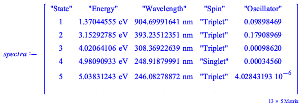 |
We can set the optional keyword showtable to true to display a fancy table of the spectra.
| > |
State |
Energy | Wavelength | Spin | Oscillator |
| Triplet | ||||
| Triplet | ||||
| Triplet | ||||
| Singlet | ||||
| Triplet | ||||
| Singlet | ||||
| Singlet | ||||
| Triplet | ||||
| Triplet | ||||
| Singlet | ||||
| Singlet | ||||
| Singlet |
The table contains information such as the excitation energy, wavelength, spin, and oscillator strength for the first 12 states. Additional or fewer states may be requested with the keyword nstates. The default method is time-dependent Hartree-Fock, but other supported methods like time-dependent density functional theory can be selected by changing the base method.
| > |
State |
Energy | Wavelength | Spin | Oscillator |
| Triplet | ||||
| Singlet |
The command ExcitationSpectraPlot generates a plot of the molecule's excitation spectra.
| > |
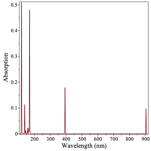 |
We can use the keyword onlysinglets to show only the excitations from the ground state to singlet excited states.
TransitionDipolePlot
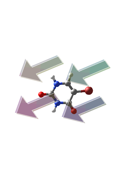
The command TransitionDipolePlot visualizes the transition dipole moment of a specified excited state.
| > |
 |
TransitionOrbitals
The command TransitionOrbitals computes the most important orbitals for the ground-to-excited-state transition using the singular value decomposition.
| > |
The singular values are returned as a vector.
| > |
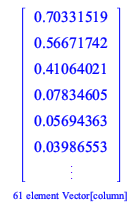 |
We observe that the first three singular values are "large" with the remaining values being negligible. The nth singular value corresponds to a transition from the molecular orbital in the corresponding column of orbital_ground to the molecular orbital in the corresponding column of orbital_excited.
TransitionOrbitalPlot
The command TransitionOrbitalPlot visualizes the pair of orbitals involved in a ground-to-excited-state transition for the nth singular value. For example, for the transition from the ground state to the first excited state, we can visualize the most important pair of orbitals associated with the first singular value.
| > |
|
Note that the change in electron density from the left (ground-state occupied orbital) to the right (excited-state occupied orbital) is consistent with the direction of the transition dipole moment (computed above).
Similarly, we can visualize the second most important pair of orbitals associated with the second singular value.
| > |
|
Again we observe that the change in electron density agrees with the direction of the transition dipole moment.
Optional Keywords
The excited-state data can also be computed directly in a supporting method. For example, we can perform a DensityFunctional computation that automatically computed the excited-state data by setting the optional keyword excited_states to true, "TDDFT" (Time-dependent Density Functional Theory) , or "TDA" (Tamm-Dancoff Approximation). Furthermore, we can control the number of computed singlet and triplet states with the optional keyword nstates whose default is 6 for 6 singlet states and 6 triplet states.
| > |
         |
The table contains entries for the excited_state_energies, excited_state_spins, transition_dipoles, oscillator_strengths, and the 1-electron reduced transition matrices (1-RTMs), for example:
| > |
| > |
 |
| > |
 |
Saving and Restoring Computations
Two new commands Save and Restore have been added to the package to make it easier than ever to save your data for future analysis. The Save command saves the cache tables associated with your calculations while the Restore command restores these cache tables in a new Maple session. This pair of commands makes it easy to switch between Maple interfaces (such as between the Maple worksheet and the Maple command-line version or between the Maple worksheet and the interactive Maplet), between operating systems (Windows, Mac OS X, or Linux), or even between different computers without redoing your computations. For advanced computations it is convenient to run computations with the Maple command-line version and then perform your analysis and visualization in the Maple worksheet (or the interactive Maplet). In the Maple worksheet or Maple document mode the commands Save() and Restore() open a directory/file browser to facilitate file selection.
Using the Package in the Classroom
The Maple Quantum Chemistry Toolbox includes many lessons that can be used in chemistry and physics courses from advanced high school courses through the graduate level. These lessons and associated curricula provide instructors and students with real-time quantum chemistry computations and visualizations that quickly deepen understanding of molecular concepts. With Maple 2020, the support for Introductory (General) Chemistry, Computational Chemistry, and Quantum Chemistry has been extended even further, with the addition of over 13 new topics, including atomic structure, chemical bonding, valence-shell electron pair repulsion (VSEPR), the Maxwell-Boltzmann distribution, heat capacity, enthalpy, entropy, free energy, as well as advanced electronic structure methods. The general chemistry lessons are ideal not only for college-level introductory chemistry courses but also secondary-school Advanced Placement (AP) and International Baccalaureate (IB) courses. Computational chemistry lessons cover electronic structure theory and methods including Hartree-Fock method, Moller-Plessett perturbation theory, density functional theory, and 2-RDM theory for use in undergraduate and graduate computational chemistry courses. In the following two subsections we show snippets of the lessons on the Maxwell-Boltzmann distribution for Introductory Chemistry and density functional theory for Computational Chemistry.
Maxwell-Boltzmann Distribution
Before we begin, we define the ideal gas constant in SI units.
| > |
We can define the Maxwell-Boltzmann distribution with Maple.
| > |  |
 |
Let us check that the total probability of the particle having some speed is unity for a gas with a molar mass of 0.1 kg/mol at a temperature of 273 K.
| > |
(a) Does the total probability equal the expected value of unity?
We can explore the Maxwell-Boltzmann distribution as a function of the temperature and molar mass of the gas.
| > |
|
|||||||||||
|
|||||||||||
Using the slide rules to change temperature T in K and molar mass M in kg/mol (SI units), answer the following questions:
(b) Approximately from the graph, what is the most probably velocity for water H2O at 275 K?
(c) Approximately from the graph, what is the most probably velocity for methane CH4 at 550 K?
Density Functional Theory
We compute the energy of diphenyl disulphide.
First, we define the geometry, which we obtained from the MolecularGeometry command.
| > |
Then we compute the energy from DFT with the DensityFunctional command. We select the B3LYP exchange-correlation (xc) functional and the 6-31g basis set.
| > |
     |
The ground-state energy is given by
| > |
(a) Compute the energy using the PBE functional, and compare your result with the energy from the B3LYP functional. Absolute energies are typically not too important in DFT.
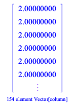
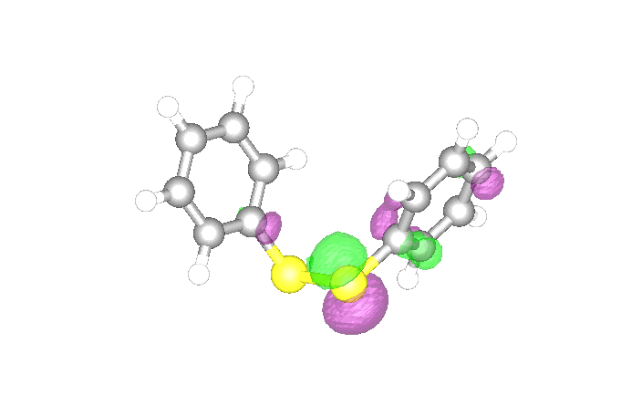
The highest occupied molecular orbital (HOMO) can be visualized with the DensityPlot3D command.
| > |
 |
| > |
 |
| > |
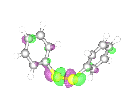 |
The energies of these two orbitals are
| > |
(b) Compare these orbitals with those from the PBE functional.