
The Regular Chains package is a collection of commands for solving systems of algebraic equations, inequations, and inequalities symbolically. It also enables users to manipulate and study the solutions of such systems. Maple's RegularChains package has received many updates since Maple 2019. Below you will find some improvements for Maple 2020.
![]()
![]()
![]()
![]()
![]()
Quantifier Elimination
Quantifier elimination is the process of taking a formula that involves statements of the form "there exists a value for variable ![]() such that..." or "for all values of variable
such that..." or "for all values of variable ![]() , we have..." (represented with the quantifiers "there exists", or
, we have..." (represented with the quantifiers "there exists", or ![]() , and "for all", or
, and "for all", or ![]() , respectively), where the rest of the statement typically involves logical connectives such as "and" or "not" and polynomial formulas, and expressing this as an equivalent statement that does not include such quantifiers but depends only on the other variables that are not quantified over. These formulas are all interpreted over the real domain.
, respectively), where the rest of the statement typically involves logical connectives such as "and" or "not" and polynomial formulas, and expressing this as an equivalent statement that does not include such quantifiers but depends only on the other variables that are not quantified over. These formulas are all interpreted over the real domain.
An example is probably in order. The following is known as the Davenport-Heintz problem:
![]()
This can be encoded as follows.
![]()
The solution is very simple. The QuantifierElimination command is in the SemiAlgebraicSetTools subpackage of RegularChains.
![]()
It is easy to see by hand that these are indeed solutions to the given problem (with e.g. ![]() in both cases), but it is not obvious that there are no other solutions.
in both cases), but it is not obvious that there are no other solutions.
We can use this functionality to find all cases where the quadratic formula has roots. We get a more legible answer by using some optional arguments to the command:
![]()
![]()
Cylindrical Algebraic Decomposition
Cylindrical Algebraic Decomposition is a partition of the real, ![]() -dimensional space into finitely many connected semi-algebraic subsets, called cells, such that any two cells are cylindrically arranged, that is, their projection onto a lower-dimensional space is either identical or disjoint. Here, a semi-algebraic set is a set given by polynomial equations, inequations, and inequalities.
-dimensional space into finitely many connected semi-algebraic subsets, called cells, such that any two cells are cylindrically arranged, that is, their projection onto a lower-dimensional space is either identical or disjoint. Here, a semi-algebraic set is a set given by polynomial equations, inequations, and inequalities.
The CylindricalAlgebraicDecompose command finds such a decomposition where the number of solutions for a given semi-algebraic system stays constant on each cell. A simple example is given as follows:
![]()
![]()
![]()
A more compact output is given with the option ![]() .
.
![]()
The ![]() command has been available for a long time. In Maple 2020, it has some new options. One of them is the optimization option. In the simplest form, it is simply a true/false option (with default value true). With this option, Maple tries to reduce the number of cells returned. This example uses the Info command, which returns a list with some information about each cell found; the number of elements of this list is the number of cells.
command has been available for a long time. In Maple 2020, it has some new options. One of them is the optimization option. In the simplest form, it is simply a true/false option (with default value true). With this option, Maple tries to reduce the number of cells returned. This example uses the Info command, which returns a list with some information about each cell found; the number of elements of this list is the number of cells.
![]()
![]()
![]()
![]()
![]()
Another change is that the default algorithm used under the hood has changed. The previous algorithm can still be selected using the method option. The default value for the method option is incremental; the other possible value is recursive. For large systems, the incremental method is typically substantially faster. In this small example, the same difference in speed occurs.
![]()
| memory used=14.99MiB, alloc change=0 bytes, cpu time=130.00ms, real time=129.00ms, gc time=0ns
|
![]()
| memory used=1.78MiB, alloc change=0 bytes, cpu time=15.00ms, real time=15.00ms, gc time=0ns
|
Computing intersection multiplicities
The new command IntersectionMultiplicity returns the intersection multiplicity of a space curve at every point of that curve defined by a regular chain. This is shown in the following example.
![]()
![]()
We consider the points of intersection of all three surfaces. First, we compute these as regular chains.
![]()
![]()
![[PIECEWISE([`+`(x, `-`(z)) = 0, ``], [`+`(y, `-`(z)) = 0, ``], [`+`(`*`(`^`(z, 2)), `*`(2, `*`(z)), `-`(1)) = 0, ``]), PIECEWISE([x = 0, ``], [y = 0, ``], [`+`(z, `-`(1)) = 0, ``]), PIECEWISE([x = 0, ...](regular-chains/RegularChains_45.gif) |
By inspection, these solutions correspond to the points ![]() (two points),
(two points), ![]() ,
, ![]() , and
, and ![]() , respectively.
, respectively.
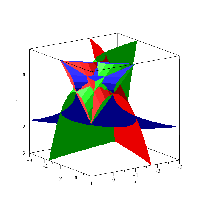
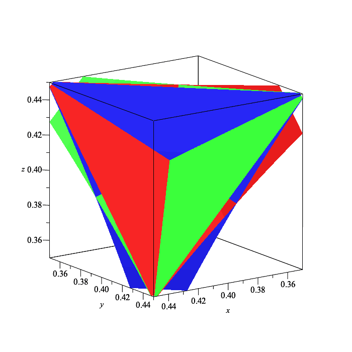
The three surfaces look as follows. We show a larger plot that includes all intersection points of all three surfaces, and two close ups: one of the point ![]() and one of the point
and one of the point ![]() .
.
![]()
 |
![]()
 |
![]() &
&
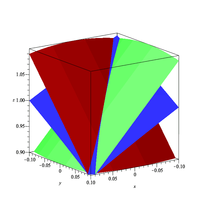 |
We see that in the second close up, the pairwise intersection curves appear to be locally tangent, which is not the case in the first close up. This is confirmed by the IntersectionMultiplicity command.
![]()
This confirms that the intersection multiplicity of all points in the first regular chain is 1, whereas it is 2 for the others.
Tangent cones
The new command TangentCone computes a tangent cone to a given space curve at a given set of points. Consider the following example.
![]()
![]()
![]() , defined above, represents the point
, defined above, represents the point ![]() .
.
![]()
We will find the tangent cone to the intersection of the surfaces defined in ![]() at the point defined in
at the point defined in ![]() . First let us examine these surfaces visually.
. First let us examine these surfaces visually.
![]()
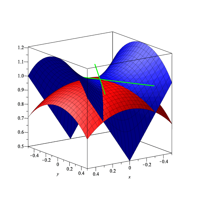
We are interested in the first and third solution. We create a plot of these two surfaces, call it ![]() , and display it.
, and display it.
![]()
 |
We now compute the tangent cone.
![]()
We see that it corresponds to the lines given by ![]() and
and ![]() . We show this in the same plot.
. We show this in the same plot.
![]()
![]()
 |
Limit points of implicitly defined curves
Another new feature of the RegularChains library is its ability to determine the geometry of curves specified as the solution set of some equations. In particular, the library can find where the leading coefficients of these equations vanish, and whether the curve is locally real at those points or not. An example follows.
Consider the equations ![]() and
and ![]() . The surfaces defined by them look as follows; this is purely for illustration and the method of drawing it won't be explained here. The first equation's surface is rendered in red, the second in blue, and the curve that is their intersection in green. You can also see a transparent black plane at
. The surfaces defined by them look as follows; this is purely for illustration and the method of drawing it won't be explained here. The first equation's surface is rendered in red, the second in blue, and the curve that is their intersection in green. You can also see a transparent black plane at ![]() , and the two intersection points of the curve with this plane in black; these are explained below.
, and the two intersection points of the curve with this plane in black; these are explained below.
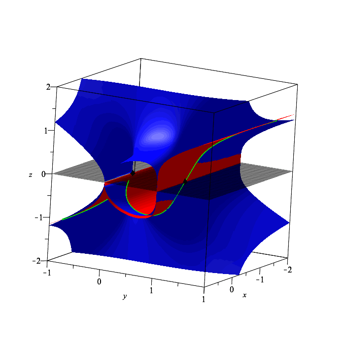 |
If we view the variables as having the order ![]() , then the leading coefficients of these equations are 1 and
, then the leading coefficients of these equations are 1 and ![]() , respectively. The first coefficient doesn't vanish; the second vanishes at
, respectively. The first coefficient doesn't vanish; the second vanishes at ![]() . The LimitPoints command can find the intersections of the curve, that is, the intersection of the red and blue surfaces. By default, this computation is done over the complex numbers.
. The LimitPoints command can find the intersections of the curve, that is, the intersection of the red and blue surfaces. By default, this computation is done over the complex numbers.
![]()
![]()
![]()
![]()
![]()
![[PIECEWISE([x = 0, ``], [y = 0, ``], [z = 0, ``]), PIECEWISE([x = 0, ``], [`+`(y, `-`(1)) = 0, ``], [z = 0, ``])]](regular-chains/RegularChains_91.gif) |
We see that there are two such limit points. Indeed, if we evaluate the polynomials defining the equations at these points, they vanish. These are the two points shown in the graph above.
![]()
![]()
It looks like there is a cusp at the origin: the curve is not smooth there. We can confirm that this is indeed the case:
![]()
 |
By using the ![]() option, we include only points where the curve is locally smooth in real space: where it locally has a Puiseux series with real coefficients. This computation uses the underlying command RegularChainBranches, which returns a truncated Puiseux series at each of these points for all branches.
option, we include only points where the curve is locally smooth in real space: where it locally has a Puiseux series with real coefficients. This computation uses the underlying command RegularChainBranches, which returns a truncated Puiseux series at each of these points for all branches.
![]()
![]()
The first two results each contain a ![]() function which represents
function which represents ![]() (or
(or ![]() ). We see that they have nonreal coefficients.
). We see that they have nonreal coefficients.
The last result is a truncated Puiseux series with only real coefficients. One might wonder if there are later terms of this series that have nonreal coefficients; but the algorithm used guarantees that this is not the case. The RegularChainBranches command can be instructed to return only truncated Puiseux series for real branches, as follows:
![]()
When we examine it in the plot, we can see that this is locally a good approximation to the intersection curve for real values of the parameter, but the other two branches are not. Indeed, the ![]() -component of the curve is nonnegative, whereas the curve is present only for
-component of the curve is nonnegative, whereas the curve is present only for ![]() . When we re-parametrize these nonreal branches by the change of variables
. When we re-parametrize these nonreal branches by the change of variables ![]() , we get the following. (The call to convert/radical converts the RootOf function into
, we get the following. (The call to convert/radical converts the RootOf function into ![]() .)
.)
![]()
![]()
Now the leading coefficient for each of the coordinates is real. Of course the (truncated) series itself can still not be embedded in real space, but we will be able to examine its real part, which should approximate the series well for small values of ![]() . Below, this real part of the truncated Puiseux series is shown in purple and the real truncated Puiseux series in pink.
. Below, this real part of the truncated Puiseux series is shown in purple and the real truncated Puiseux series in pink.
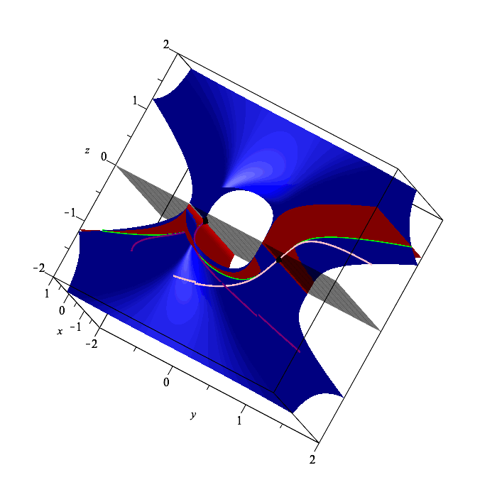 |