
2-D Cross-Correlation
The SignalProcessing package has been enhanced with a new command for the cross-correlation of matrices, CrossCorrelation2D.
A classic application of two-dimensional cross-correlation is the lining up of two or more images, for example, images of fingerprint fragments. Consider the following image:
| > | restart:
with( SignalProcessing ): with( ImageTools ): |
| > | fingerprint := Matrix( Read( cat( kernelopts( mapledir ), kernelopts( dirsep ), data, kernelopts( dirsep ), "images", kernelopts( dirsep ), "fingerprint.jpg" ) ) ): |
| > | Preview( fingerprint ); |
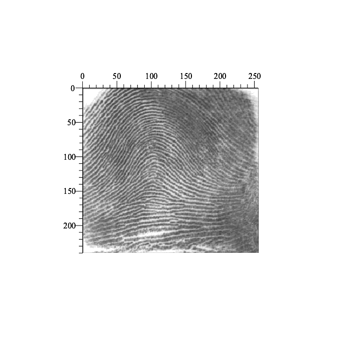 |
First, determine the dimensions and calculate the mean:
| > | a, b := upperbound( fingerprint );
mu := add( fingerprint ) / numelems( fingerprint ): |
| (1.1) |
Second, let's choose bounds for a fragment of the fingerprint, extract the sub-image (fingerprint fragment), and then add noise (to make our task a little more realistic):
| > | cL := 85:
cU := 205: dL := 120: dU := 180: fingerprint_part := fingerprint[ cL..cU, dL..dU ] + 0.5 * mu * ArrayTools:-RandomArray( cU-cL+1, dU-dL+1, distribution = normal ): Preview( fingerprint_part ); |
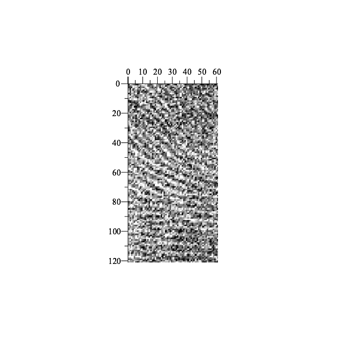 |
Suppose now that we do not know whether the fragment is part of the larger image, and wish to determine if the fragment is a "match". To do this, compute the cross-correlation of the tempered data (formed by subtracting the mean from all elements):
| > | mu := add( fingerprint ) / numelems( fingerprint ): |
| > | C := map( Re, CrossCorrelation2D( fingerprint -~ mu, fingerprint_part -~ mu ) ): |
The maximum correlation occurs here, which, as expected, coincides with the bottom-right corner of the fragment:
| > | alpha, beta := max[index]( C ); |
| (1.2) |
Convolution with Complex Signals
The SignalProcessing:-Convolution command now supports signals with complex elements. For example:
| > | A := Array( [1-2*I,3+4*I], datatype = complex[8] );
B := Array( [5-6*I,7+8*I,9-10*I], datatype = complex[8] ); |
| (2.1) |
| > | C := SignalProcessing:-Convolution( A, B ); |
| (2.2) |
A container for storing the complex Array can also be passed:
| > | Z := Array( 1 .. 4, datatype = complex[8] ):
SignalProcessing:-Convolution( A, B, container = Z ): 'Z' = Z; |
| (2.3) |
Hough Transform and Probabilistic Hough Transform
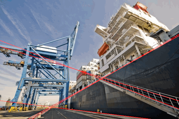
The new HoughLine and ProbabilisticHoughLine commands are used to detect straight lines in images using the Hough Transform.
First define two procedures that draw lines and line segments across an image
| > | DrawLine := proc(img, line)
local i, nRows, nCols, rho, theta, pixel, x1, y1, x2, y2; nRows := upperbound(img, 1); nCols := upperbound(img, 2); pixel := nRows + nCols; for i to upperbound(line, 1) do rho := line[i, 1]; theta := line[i, 2]; x1 := rho * cos(theta) - pixel * sin(theta); y1 := rho * sin(theta) + pixel * cos(theta); x2 := rho * cos(theta) + pixel * sin(theta); y2 := rho * sin(theta) - pixel * cos(theta); Draw:-Line(img, x1, y1, x2, y2, [255, 0, 0]): end do; end proc: DrawLineSegment := proc(img, line) local i; for i to upperbound(line, 1) do Draw:-Line(img, line[i, 1], line[i, 2], line[i, 3], line[i, 4], [255, 0, 0]); end do; end proc: |
Import an image
| > | img := Read(cat( kernelopts( mapledir ), kernelopts( dirsep ), data, kernelopts( dirsep ), "images", kernelopts( dirsep ), "ship.jpg" )):
Embed(img) |

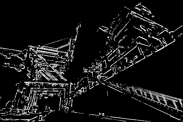
Hough transforms work best on an image that has been processed with an edge detection routine, and then binarized with respect to a threshold.
| > | edge := Threshold(EdgeDetect(img, method = Prewitt4), 5.5):
Embed(edge) |
| > | line := HoughLine(edge, 1, Pi/180, 200) |
![rtable(1 .. 5, 1 .. 2, [[149.0, 1.8675023317337036], [396.0, 1.0646508932113647], [127.0, 1.9373154640197754], [400.0, 1.0471975803375244], [336.0, 1.6929693222045898]], subtype = Matrix);](signalimageprocessing/SignalImageProcessing_11.gif) |
(3.1) |
| > | imgv := Flip(img, 'vertical'):
DrawLine(imgv, line); Embed(Flip(imgv, 'vertical')); |
| > | line := ProbabilisticHoughLine(edge, 1, Pi / 180, 10, 100, 10); |
![_rtable[18446746025195752854];](signalimageprocessing/SignalImageProcessing_13.gif) |
(3.2) |
Flip the image as the origin for Draw:-Line is on the bottom-left corner
| > | DrawLineSegment(img, line);
Embed(img); |

2D Haar Wavelet Transforms
The new ImageTools:-DWT2D and ImageTools:-InverseDWT2D commands compute the Haar wavelet of grayscale or color image.
| > | result := DWT2D(fingerprint, level = 1):
approx, horiz_detail, vert_detail, diag_detail := map(rtable, result, datatype = float[8])[]: |
| > | Embed( << < approx | horiz_detail >, < vert_detail | diag_detail > >>) |
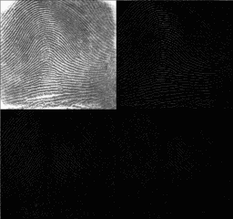
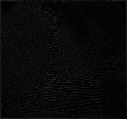
Zero out the approximation, but leave the horizontal, vertical and diagonal details as is.
| > | approxSize := ArrayTools:-Size(approx) |
| (4.1) |
| > | approx_new := Array(1..approxSize[1], 1..approxSize[2], fill = 0.0, datatype = float[4]): |
Now reconstruct the image with an inverse wavelet transform.
| > | res2 := InverseDWT2D([approx_new, horiz_detail, vert_detail, diag_detail]): |
| > | Embed(Create(res2)) |
Hilbert Transform
The Hilbert command in the SignalProcessing package is the discrete version of the corresponding integral transform. For example:
| > | X := map[evalhf]( t -> 10 / (t^2+1), Vector[row]( < seq( -10 .. 10, 0.25 ) >, datatype = float[8] ) ): |
| > | H := Hilbert( X ): |
| > | dataplot(
[Re,Im]( H ), legend = ["Original signal","Transformed signal"], title = "Discrete Signals vs. Index", color = [blue,red], symbolsize = 7, font = [Verdana,15], legendstyle = [font=[Verdana,10]] ); |
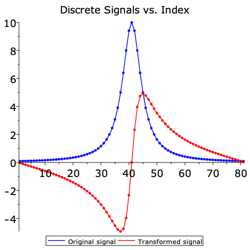 |
Note that the result is a complex signal, with the real part being the original signal, and the imaginary part being the transformed signal.
Root Mean Square (RMS)
The new RootMeanSquare command provides a way to measure the size of a 1-D signal:
![RootMeanSquare(A) = sqrt(`/`(`*`(Sum(`*`(`^`(abs(A[i]), 2)), i = 1 .. n)), `*`(n)));](signalimageprocessing/SignalImageProcessing_19.gif) , where
, where ![]()
For example:
| > | with( SignalProcessing ): |
| > | RootMeanSquare( < 2, 2, 2, 2 > ); |
| (6.1) |
| > | RootMeanSquare( < 5, -3, 7.5, 2 > ); |
| (6.2) |
We can also measure how close two signals are to each other. Here, we compare a signal with the Inverse Discrete Fourier Transform (IDFT) of its Discrete Fourier Transform (DFT):
| > | A := LinearAlgebra:-RandomVector( 100, datatype = complex[8] ):
B := DFT( A ): C := InverseDFT( B ): RootMeanSquare( A - C ); |
| (6.3) |
Furthermore, we can see that the RMS for both the signal and its DFT are the same (Parseval's Theorem):
| > | abs( RootMeanSquare( A ) - RootMeanSquare( B ) ); |
| (6.4) |