Visualization - New Features in Maple 2020 - Maplesoft

What's New in Maple 2020

Visualization

Maple 2020 includes the following visualization updates.


Plot size 

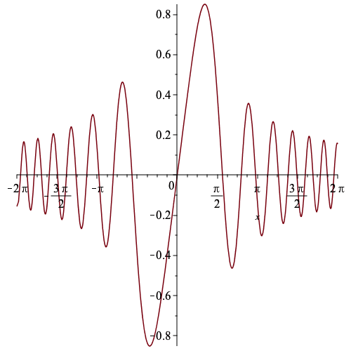
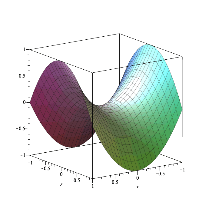
The default plot size for 2-D and 3-D plots is bigger, for better visibility on high resolution monitors. 

`/`(`*`(sin(`*`(`^`(x, 2)))), `*`(x)); Plot_2d 

plot3d(`+`(`*`(`^`(x, 2)), `-`(`*`(`^`(y, 2)))), x = -1 .. 1, y = -1 .. 1);

Plot_2d

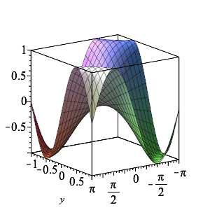
In addition, the size option is now supported for 3-D plotting commands.  This allows for specifying precise and consistent dimensions for the plotting window that encapsulates inline 3-D plots. This geometry is respected upon export of the plot to an image file. 

The size option is also supported by the plots:-display command for combining multiple 3-D plots. 

plot3d(sin(`*`(x, `*`(y))), x = `+`(`-`(Pi)) .. Pi, y = -1 .. 1, size = [300, 300]);  

Plot_2d
 

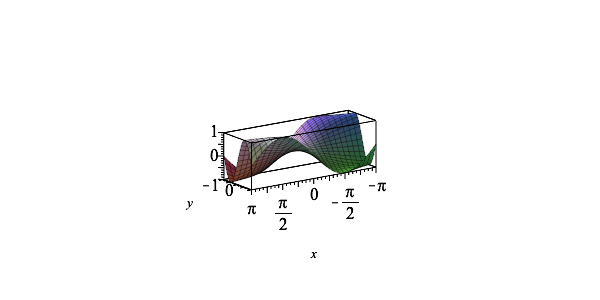
The following plot has also been manually zoomed and panned. 

plot3d(sin(`*`(x, `*`(y))), x = `+`(`-`(Pi)) .. Pi, y = -1 .. 1, scaling = constrained, size = [600, 300]);

Plot_2d

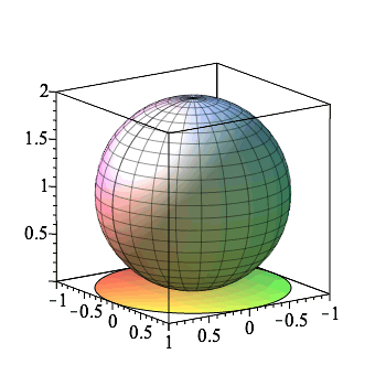
with(plottools); -1; plots:-display(sphere([0, 0, 1], 1), (transform(proc (x, y) options operator, arrow; [x, y, 0] end proc))(disk([0, 0], 1)), size = [350, 350])

Plot_2d


Legends for 2-D contour plots 

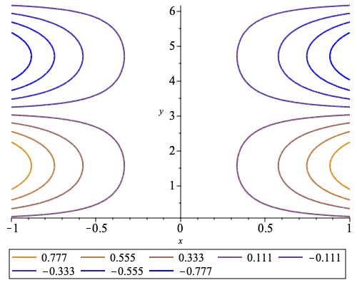
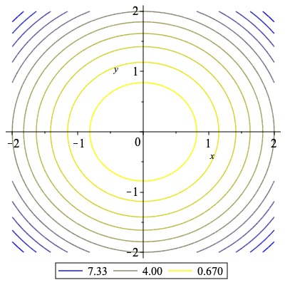
The plots:-contourplot command's support for the legend option now allows for both automatic generated and customized legend entries to display the values of the contour lines.

with(plots); -1 

contourplot(`*`(`^`(x, 2), `*`(sin(y))), x = -1 .. 1, y = 0 .. `+`(`*`(2, `*`(Pi))), thickness = 2, coloring = [ 

Plot_2d


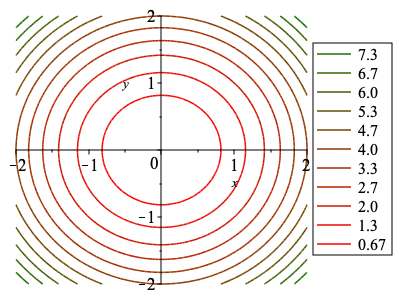
When supplied as a list the number of legend entries must match the requested number of contour lines.  The contour values can be numerically formatted.
 

contourplot(`+`(`*`(`^`(x, 2)), `*`(`^`(y, 2))), x = -2 .. 2, y = -2 .. 2, contours = 11, coloring = [
 

Plot_2d


The special name
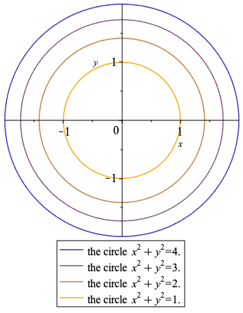
contourvalue can be used within a typeset formula.
 

contourplot(`+`(`*`(`^`(x, 2)), `*`(`^`(y, 2))), x = -2 .. 2, y = -2 .. 2, contours = [seq(i, i = 1 .. 4)], coloring = [
 

Plot_2d


The special value
"null" can be used to suppress the legend entry for particular contours.
 

contourplot(`+`(`*`(`^`(x, 2)), `*`(`^`(y, 2))), x = -2 .. 2, y = -2 .. 2, coloring = [
 

Plot_2d


Adaptive edge computation for plot3d

The new adaptmesh option of the plot3d command provides for automatic adjustment of the independent values of the data points in order to display smoother edges for surfaces which are non-numeric in some part of the specified rectangular domain.

In previous releases, the surface appeared as it now does with the option given as
adaptmesh=false. The new default behavior is adaptmesh=true. In the following two graphs, the default behavior in Maple 2020 is shown on the right.
 

expr := `+`(`/`(1, 2), `-`(`*`(`/`(1, 10), `*`(x))), sqrt(`+`(`-`(`*`(`^`(x, 2))), `-`(`*`(`^`(y, 2))), 1)), `*`(`/`(1, 2), `*`(sqrt(`+`(`*`(`^`(`+`(y, `/`(1, 2)), 2)), `*`(`^`(`+`(x, `-`(`/`(1, 3))),...
 

plots:-display(Array([plot3d(expr, rng, opts, adaptmesh = false), plot3d(expr, rng, opts, adaptmesh = true)])); 1 

Plot_2d Plot_2d


expr := proc (x, y) options operator, arrow; `+`(`-`(`*`(x, `*`(`^`(y, 2), `*`(sqrt(`+`(1, `-`(`*`(2, `*`(`^`(x, 3)))), `-`(`*`(`^`(y, 3)))))))))) end proc; -1; rng := -1 .. 1, -1 .. 1; -1; opts := co...
 

Plot_2d Plot_2d


With the option set to true the result contains a MESH structure, while with the option set to false the result contains a GRID structure.

The data values can still be extracted using the
plottools:-getdata command.
 

op([1, 0], old), op([1, 0], new); 1 

GRID, MESH
 

interface(rtablesize = 3); -1 

plottools:-getdata(old); 1 

[
 

plottools:-getdata(new); 1 

[
 

interface(rtablesize = 10); -1 


plottools[triangulate] 

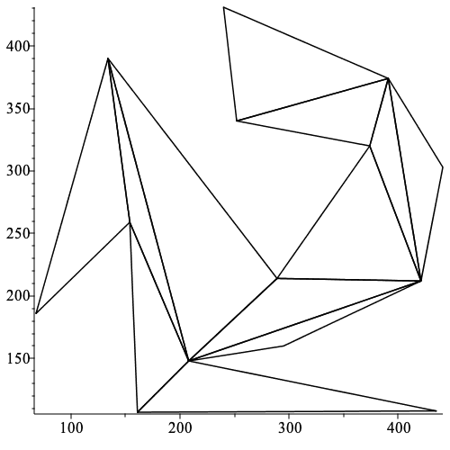
The triangulate command takes a POLYGONS or POINTS structure and return a POLYGONS structure containing a set of triangles which cover the region defined by its input. 

pts := [[391, 374], [240, 431], [252, 340], [374, 320], [289, 214], [134, 390], [68, 186], [154, 259], [161, 107], [435, 108], [208, 148], [295, 160], [421, 212], [441, 303]]; -1
 

P := plottools:-polygon(pts); -1 

Q := plottools:-triangulate(P, style = line);  

Typesetting:-mrow(Typesetting:-mi(
 

plots:-display(Q);  

Plot_2d


ColorTools:-CVDSimulation 

CVDSimulation in the ColorTools package is a new command that returns how a color could be perceived by a viewer with a specific color vision deficiency. 

> with(ColorTools); -1
 

> P := GetPalette(
 

Typesetting:-mrow(Typesetting:-mrow(Typesetting:-mi(
 

> `~`[CVDSimulation](P,
 

_rtable[18446746203458510846];
 

> `~`[CVDSimulation](P,
 

_rtable[18446746203555937446];
 

> `~`[CVDSimulation](P,
 

_rtable[18446746203561641254];