Example: Visualizing an Optimization Problem in Parallel	Integrated Local Grid Computing

In this example we want to optimize a nonlinear constraint problem. Instead of just getting a final number from a black-box routine, we want to look at the constraints and visualize partial solutions. The following problem is described by Rakesh Angira and B.V. Babu in section 6 of the paper "Optimization of Non-Linear Chemical Processes using Modified Differential Evolution". The goal is to determine the optimal operation of an alkylation unit, commonly used in the petroleum industry.

The objective function is described as a function of total profit.



The constraints are written in terms of: olefin feed rate (x1), acid addition rate (x2), alkylate yield (x3), acid strength (x4), motor octane number (x5), external isobutane-to-olefin ratio (x6), and F-4 performance number (x7).





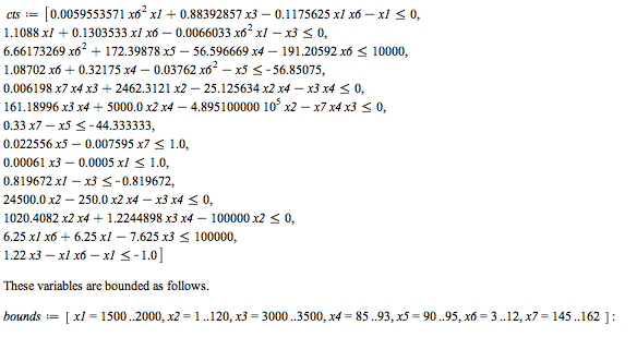
Parameter Sweep

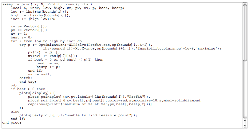
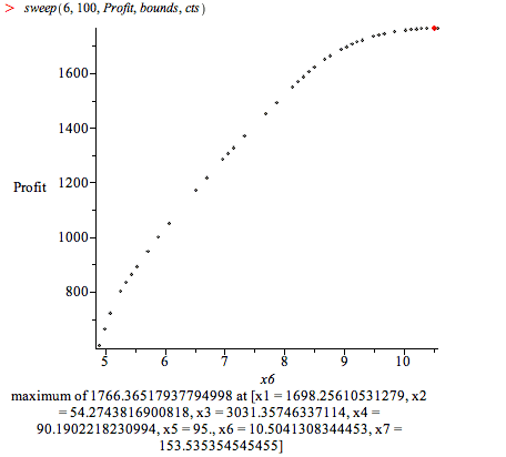
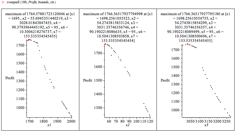
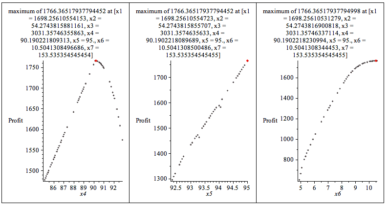
Looking at the equations, you can see that x6 terms are raised to the power 2 in some cases. This variable likely has a big effect on the answer. It would be good to see how the total profit varies with x6. You can use Maple's built-in nonlinear local solver to sweep over a range of feasible values for x6. Define a procedure that accepts the index of the variable you want to analyze and the number of points you want to sample.



Call the above procedure on the 6th variable with 100 sample points:



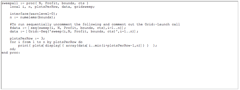
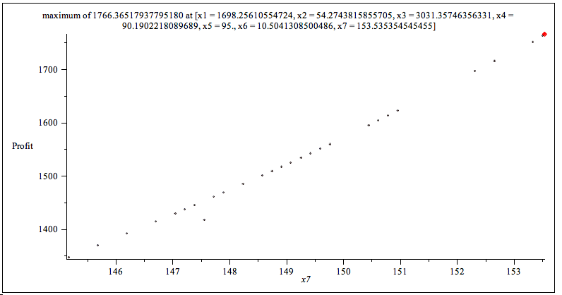
Write a second procedure that sweeps over all of the variables and outputs plots side-by-side. The code in this procedure is structured so it can be run in parallel.







Refining the Constraints
It is clear from the plots where the boundary constraints can be refined, thereby simplifying the example. Try redefining the boundaries and running another sweep.

bounds2 := [x1 = 1685 .. 1730, x2 = 1 .. 59, x3 = 3020 .. 3045, x4 = 89.6 .. 92, x5 = 94.8 .. 95, x6 = 9 .. 12, x7 = 153 .. 162] :

sweepall(150, Profit, bounds2, cts);





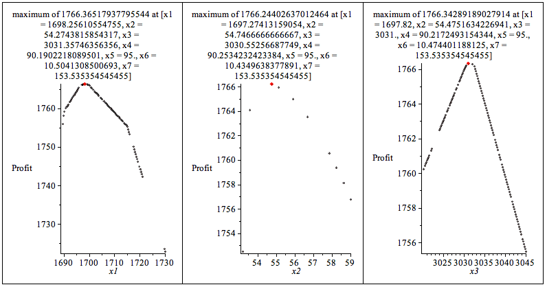
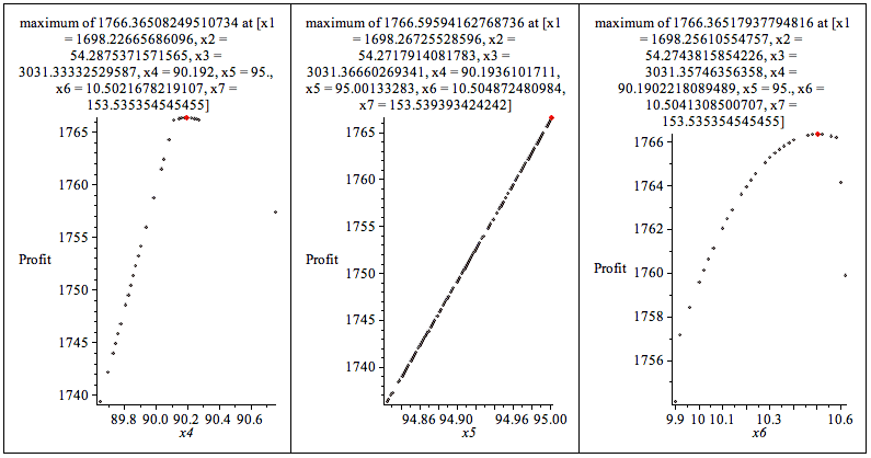
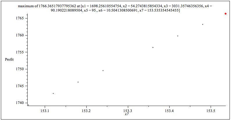
Clearly we are narrowing in on the optimal value, and gaining a good sense of how changing the parameters will affect the result. By reviewing the initial constraints, you can change the process so the bounds of a particular variable are made wider. For example, by increasing the allowed bounds of x5 by less than 1%, the total maximum profit can be increased by more than $100.

If you blinked, you may not have noticed that the only change required was to swap a call to seq with a call to Grid:-Seq. After that, the code uses all the power of your local computer, and delivers results in a fraction of the time.

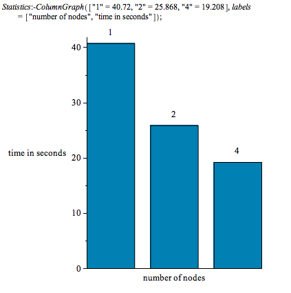
Execution time on a 2-core Intel Core i5-M560 Windows 7 laptop. Due to hyperthreading, performance continues to improve on 4 nodes even though this laptop only has 2 cores.

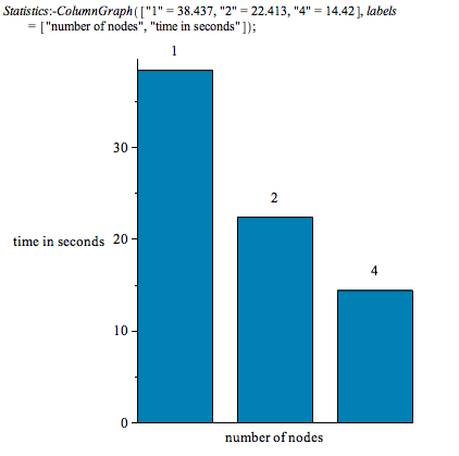
Execution time on a 4-core Intel Core 2 Quad Q8200 desktop. ; Timings were computed using the time[real] command to measure elapsed time (not CPU time), using 500 sample points, and include time taken to display the plots.

Integrated Local Grid Computing