Introduction
Maple 17 offers new signal processing tools for analyzing and manipulating data in the frequency and time domains. It can be used for diverse applications such as creating a speech spectrogram, removing noise from polluted signals, and identifying the periodicity of data.
This package includes tools for:
- Cosine, fast Fourier and wavelet transforms
- Bartlett, Blackman, Kaiser, Hann, and Hanning windows
- Signal generation
- Cross-correlation, autocorrelation, data statistics, and upsampling/downsampling
- FIR, IIR, and Butterworth filters
| > |
![with(SignalProcessing[Engine])](/products/maple/new_features/images17/SignalProcessing/SignalProcessing_2.gif) |
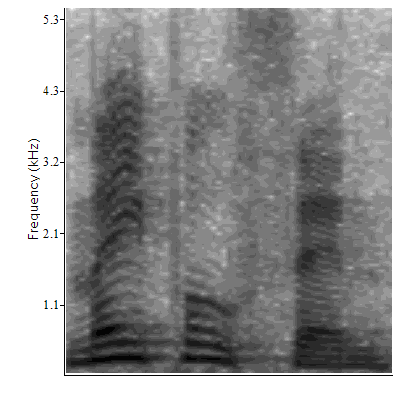
Application: Imaging a Speech Spectrogram
Import Wave File and Manipulate Data into Overlapping Slices
| > |
 |
| > |

 |
| > |
 |
| > |
  |
| > |
 |
Slice the data into segments with 256 samples. Each slice has a 50% overlap with the previous slice (that is, each slice starts at the half-way point of the previous slice).
| > |
 |
| > |
 |
| > |
![sample := Matrix(samps, nTimes, proc (i, j) options operator, arrow; data[`+`(i, `*`(`/`(1, 2), `*`(`+`(j, `-`(1)), `*`(samps))))] end proc, datatype = float[8]); 1](/products/maple/new_features/images17/SignalProcessing/SignalProcessing_25.gif) |
Calculate the Spectrogram Data
Filter the data, slice by slice.
| > |
![a := `<|>`(`<,>`(seq(HannWindow(sample[() .. (), i]), i = 1 .. nTimes))); -1](/products/maple/new_features/images17/SignalProcessing/SignalProcessing_27.gif) |
Calculate FFT of time segment consecutively.
| > |
![FFTa := `<|>`(`<,>`(seq(FFT(a[i, () .. ()]), i = 1 .. nTimes))); -1](/products/maple/new_features/images17/SignalProcessing/SignalProcessing_28.gif) |
Calculate Power Spectrum of each slice consecutively.
| > |
 .. ()])), i = 1 .. nTimes))); -1](/products/maple/new_features/images17/SignalProcessing/SignalProcessing_29.gif) |
Convert spectrum into decibels.
| > |
 |
| > |
 |
Strip out the repeated data.
| > |
 |
| > |
 |
The frequencies go from 0 to half the sampling rate. Hence the frequencies are in steps of (in Hz):
| > |
 |
Scale the spectra so that the values are between 0 and 255.
| > |
 |
| > |
 |
| > |
 |
Consecutive rows represent slices in time, while columns contain the spectra at each time.
| > |
; 1](/products/maple/new_features/images17/SignalProcessing/SignalProcessing_42.gif) |
Plot the Spectrogram and Waveform
| > |
![commonPlotOpts1 := labelfont = [Helvetica], labeldirections = [horizontal, vertical]; -1](/products/maple/new_features/images17/SignalProcessing/SignalProcessing_44.gif) |
| > |
![p2 := listplot([seq([`/`(`*`(i), `*`(samplingRate)), data[i]], i = 1 .. numelems(data))], thickness = 0, gridlines, axes = boxed, labels = [](/products/maple/new_features/images17/SignalProcessing/SignalProcessing_48.gif)
![p2 := listplot([seq([`/`(`*`(i), `*`(samplingRate)), data[i]], i = 1 .. numelems(data))], thickness = 0, gridlines, axes = boxed, labels = [](/products/maple/new_features/images17/SignalProcessing/SignalProcessing_49.gif) |
| > |
![display(Array(`<|>`(`<,>`(p1, p2))), aligncolumns = [1])](/products/maple/new_features/images17/SignalProcessing/SignalProcessing_50.gif) |
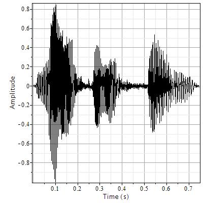
Application: Filtering Audio
Import Speech Sample
| > |

 |
| > |
 |
Plot Waveform and Power Spectrum
| > |
![commonPlotOpts2 := titlefont = [Helvetica, 12], labelfont = [Helvetica], labeldirections = [horizontal, vertical], axis = [gridlines = [color =](/products/maple/new_features/images17/SignalProcessing/SignalProcessing_58.gif)
![commonPlotOpts2 := titlefont = [Helvetica, 12], labelfont = [Helvetica], labeldirections = [horizontal, vertical], axis = [gridlines = [color =](/products/maple/new_features/images17/SignalProcessing/SignalProcessing_59.gif) |
| > |
![samplingRate := attributes(originalSpeech)[1]](/products/maple/new_features/images17/SignalProcessing/SignalProcessing_60.gif) |
| > |
 |
| > |
 |
| > |
![fq := FFT(originalSpeech[1 .. `^`(2, 15)]); -1](/products/maple/new_features/images17/SignalProcessing/SignalProcessing_71.gif) |
| > |
 |
| > |
 |
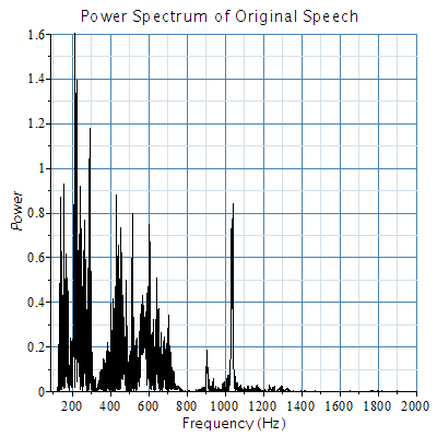
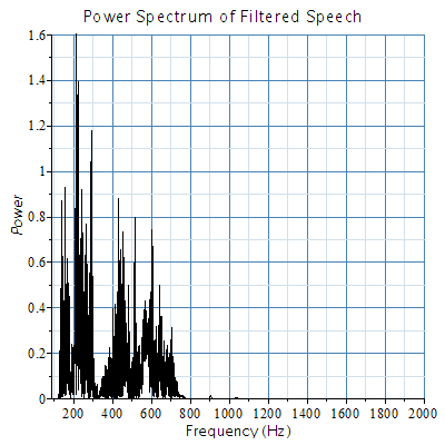
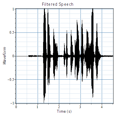
Apply IIR Butterworth or Chebyshev Filter
Apply Filter
| > |
 |
| > |

 |
| > |
 |
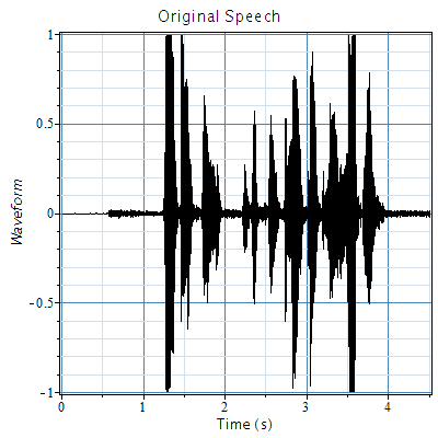
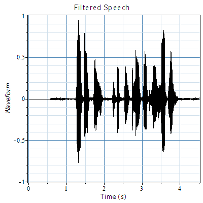
View Before and After Power Spectrum and Waveform
| > |
![FFTfilteredSpeech := FFT(filteredSpeech[1 .. `^`(2, 15)]); -1](/products/maple/new_features/images17/SignalProcessing/SignalProcessing_84.gif) |
| > |
 |
| > |
 |
| > |
![plots:-display(Array(`<,>`(`<|>`(p1, p2))), view = [0 .. duration, -1 .. 1])](/products/maple/new_features/images17/SignalProcessing/SignalProcessing_96.gif) |
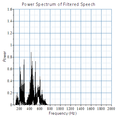
Apply FIR Filter
Apply Filter
| > |
 |
| > |
 |
| > |

 |
| > |
 |
View Before and After Power Spectrum and Waveform
| > |
![FFTfilteredSpeech := FFT(filteredSpeech[1 .. `^`(2, 15)]); -1](/products/maple/new_features/images17/SignalProcessing/SignalProcessing_104.gif) |
| > |
 |
| > |
 |
| > |
![plots:-display(Array(`<,>`(`<|>`(p1, p2))), view = [0 .. duration, -1 .. 1])](/products/maple/new_features/images17/SignalProcessing/SignalProcessing_116.gif) |

](/products/maple/new_features/images17/SignalProcessing/SignalProcessing_16.gif)
](/products/maple/new_features/images17/SignalProcessing/SignalProcessing_26.gif)
](/products/maple/new_features/images17/SignalProcessing/SignalProcessing_43.gif)
](/products/maple/new_features/images17/SignalProcessing/SignalProcessing_57.gif)


](/products/maple/new_features/images17/SignalProcessing/SignalProcessing_82.gif)