New Features in Maple 17 – Statistics

New Features in Maple 17: Statistics

Maple contains a wealth of functionality for doing statistics, combining the ease of working in a high-level, interactive environment with a very large and powerful set of algorithms. Support for statistics has been further expanded in Maple 17. The new release includes:

A new algorithm for fitting data in an overdetermined system for use in predictive models.
New robust measure of dispersion that is more suitable for asymmetric distributions than the median absolute deviation.

Fitting Data for Use in a Predictive Model

Maple 17 has a new algorithm for fitting data in an overdetermined system for use in predictive models.

Consider a survey of large-cap Energy sector stocks in the S&P 500, where you know a lot of information about a few listings. Assume in this case that most of the data, when adjusted against general market trends, ends up being useless for predicting future markets, but some properties do end up being strong market indicators. You do not, however, know which variables to keep and which not to.

Let's set up an example using random data to model this situation.

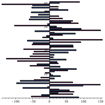
At this point we have generated the known data, and have profit numbers for that data. The following chart takes one sample parameter, property 10, and plots it against the profit. It is not obvious what the correlation is.

Plot_2d

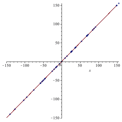
We want to build a model that fits all 100 properties against the data. A least-squares fit is used for comparison.

Because there are more variables than observations, we'll always get a perfect fit with 100% correlation to the existing data.

We don't really want a model that will perfectly fit today's data. We want a model that will detect which parameters are likely to actually correlate well with the profit observed and can be used in predicting new observations. We want to avoid overfitting.

Plot_2d

Let's set up a new model using predictive least-squares.

Note that the PredictiveLeastSquares command, new in Maple 17, returns two things: the coefficient matrix (as with regular least-squares) as well as a list indicating the columns of data that it decided were most relevant for use in predicting data.

The correlation with the current profit data is not perfect (as expected) but still very good.

Plot_2d

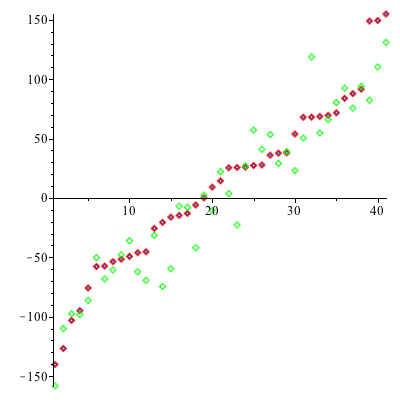
The following graph shows the standard least-squares (red), predictive least-squares (green), and actual numbers on the same plot.

Plot_2d

These commands also illustrate another new feature of Maple 17: the output option for sort. It can be used to obtain the reordering applied to the input (in this case, ) in order to sort it. This reordering (in this case, ) can then, for example, be applied to other lists or vectors, as is the case here.

Now we will generate some further data based again on the same hidden indicators, of which only some actually appear as items in the data that we know about.

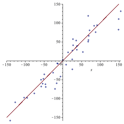
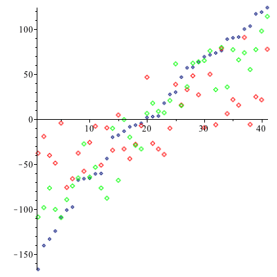
Let's first use the standard least-squares model against the new data.

It is clear that the model suffers from overfitting against spurious parameters in the original data set.

The predictive model achieved a much better correlation when using new data.

Plot_2d

It is clear that the predictive least-squares data (green) more closely matches the actual points in black, whereas the standard least-squares data (red), which generally correlates, is much more scattered.

Robust Measures of Dispersion

A measure of dispersion is a statistic of a data set that describes the variability or spread of that data set. Two well-known examples are the standard deviation and the interquartile range. Maple 17 introduces a new measure of dispersion called Sn, originally proposed by Rousseeuw and Croux [1].

Let us investigate how measures of dispersion behave when noise is added to a data set. Specifically, we will have an original data set of, say, data points, and a perturbed data set where a certain fraction of the data points are changed dramatically. We investigate at what value of the values become meaningless.

X := Vector[column](%id = 18446744078088537382)

Y := Vector[column](%id = 18446744078088537502)

For the standard deviation, we see that changing only one data point can massively change the standard deviation. In other words, there is no positive fraction of the data points that we can change while keeping the standard deviation bounded. We say that the breakdown point of the standard deviation is 0.

For the interquartile range, the process is different. Changing a single data point doesn't make the interquartile range of change very much; in fact, we can change up to a quarter of the data points while staying within an order of magnitude from the interquartile range of . As soon as we have changed 250 out of the 1000 data points, though, the interquartile range also goes through the roof.

Y := Vector[column](%id = 18446744078088537622)

> Y

This suggests that the breakdown point of the interquartile range is : changing strictly fewer than of the points cannot make the interquartile range unbounded. This is indeed correct. We say that the interquartile range is more robust than the standard deviation.

The breakdown point for any statistic can never be more than : if we change over half of the data points in the set, then there's no way to decide what the "correct" data is, and what the "changed" data is. So are there dispersion statistics that reach this maximal breakdown point?

Yes, there are. A relatively well-known one is the median absolute deviation from the median, available in Maple as MedianDeviation. As the name says, it is obtained by computing the absolute difference between every data point and the median of the data set, and taking the median of these values.

The median absolute deviation from the median is a very useful robust estimator, but it also has some disadvantages, explained in the paper [1] by Rousseeuw and Croux. One of their objections is that it doesn't deal with asymmetric distributions very well, and another is that, while it is very robust against extreme changes in some points, it needs relatively many data points to "converge" to the proper value for a distribution in the absence of disturbance. In the statistics literature, this is phrased as saying that the median absolute deviation from the median is not very efficient. 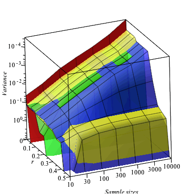These authors propose two alternative statistics that also have a breakdown point of but higher efficiency, called and . Maple 17 has an implementation of , which is called RousseeuwCrouxSn. This is a new command for Maple 17.

We will show how all of these statistics deviate from their true value for beta-distributed data samples at sample sizes from 10 to 10000 and with fractions between and of the data replaced by the value . In particular, given the sample size and the fraction , we replace the highest percent of the data by , then divide value obtained for the changed sample by the true value for the distribution, thus obtaining a number that should be for an ideal statistic. We then repeat this times, and take the average squared difference from . This is the number shown in the plot below for each of the four measures of dispersion discussed above.

results := Vector[column](%id = 18446744078088538102)

Plot_2d

The colors are red for the standard deviation, green for the interquartile range, blue for the median absolute deviation from the median, and yellow for Rousseeuw and Croux' . Lower numbers are shown higher in the graph, and are better. We see that in the case where there is no distortion (), the standard deviation has the lowest distortion. However, as soon as there is any distortion, it is immediately too inaccurate to be useful for any purpose. For , the interquartile range (green) does reasonably well, but greater values of make it, too, unusable. The median absolute deviation from the median (in blue) and (yellow) are pretty close in most cases, with yellow coming out on top slightly more often than blue. We see that is a good choice for a robust statistic of dispersion.

References

Rousseeuw, Peter J., and Croux, Christophe. Alternatives to the Median Absolute Deviation. Journal of the American Statistical Association 88(424), 1993, pp.1273-1283.

Differential Geometry