New Features in Maple 17 – Control Design

New Features in Maple 17: Control Design

Control design tools in Maple have been enhanced to become even more flexible. Improvements to the DynamicSystems package include:

The FrequencyResponse routine handles differential equations with input derivatives.
All models now accept linear, non-differential systems.
A new frequencies option for all frequency-based plots enables you to specify the precise frequencies at which expressions are evaluated.
The Grammians command has been extended to work with discrete systems.
Nichols plots are now accessible from the context-sensitive menu.

Example

Assign a differential system with derivatives in the input.

Plot the magnitude of the response vs frequency, adding circles at selected frequencies. This is done by generating and combining two plots.

Plot_2d

Example

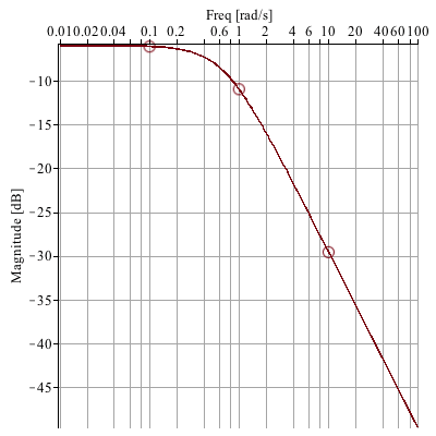
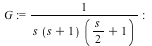
A Nichols plot is useful for quickly estimating the closed-loop response of system with unity-feedback, given its open-loop transfer function. For example, let the open-loop transfer function be:

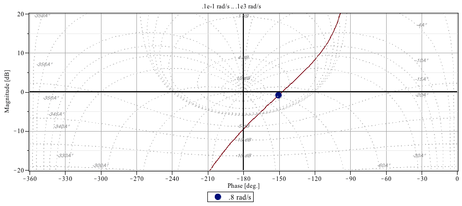
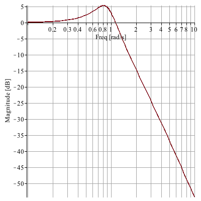
By default a Nichols plot includes constant-phase and constant-magnitude contour plots of a closed-loop system. From the graph below, the peak closed-loop response is about 5 dB, at 0.8 rad/s, because that is the highest constant-magnitude contour that it touches (estimating).

Plot_2d

Here we plot the actual closed-loop response and confirm that the maximum gain is approximately 5 dB, at 0.8 rad/s.

Plot_2d

Visualization