|
Algebraic Riccati equations appear in many linear optimal and robust control methods such as in LQR, LQG, Kalman filter, H2 and H ∞ techniques. Solving these equations is a vital step in designing such controllers and state estimators. In Maple 15, the CARE and DARE solvers for continuous and discrete algebraic Riccati equations are enhanced with high-precision solvers that allow you to get solutions beyond IEEE double precision.
One of the main methods in linear optimal control theory is the Linear Quadratic Regulator (LQR) in which a state feedback law is designed to minimize a quadratic cost function. In continuous-time domain, the optimal state feedback gain, K, is calculated such that the quadratic cost function

is minimized by the feedback law u = -Kx subject to the system dynamics 
The calculated feedback law stabilizes the closed loop system. That is, for every nonzero initial condition, the states of the closed loop system asymptotically converge to the origin. Q and R are weighting matrices over the states and inputs, respectively, balancing the optimization between the speed of convergence and the required control effort.
The optimal LQR state feedback gain is given as:

where X is the solution of the following continuous-time algebraic Riccati equation (CARE):

Similarly, in discrete-time domain, the optimal state feedback gain, K, is calculated such that the quadratic cost function

is minimized by the feedback law u[n] = -Kx[n] subject to the system dynamics

The optimal LQR state feedback gain is given as:

where X is the solution of the following discrete-time algebraic Riccati equation (DARE):

In order for the LQR problem to be solvable,
- The pair (A, B) must be stabilizable.
- The pair (Q, A) must have no unobservable modes on the imaginary axis in continuous-time domain or on the unit circle in discrete-time domain.
- R > 0 (positive definite) and Q ≥ 0 (positive semidefinite).
Example
This example shows a problem that cannot be solved using IEEE double precision, but can be solved with Maple 15's unlimited precision solvers.

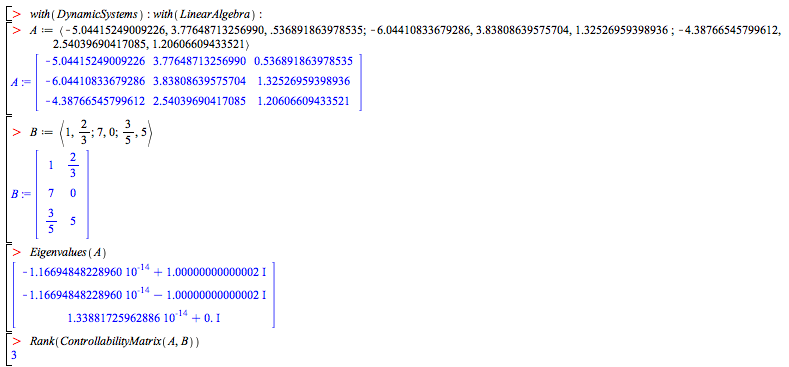
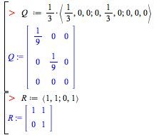
The system is not asymptotically stable but the pair (A,B) is controllable. Suppose, the weighting matrices are given as

Note that R is not symmetric but it is positive definite. This can be verified as follows:

The (Q,A) pair is observable:

The CARE solver is called and the ouput option is set to directly return the LQR gain:

An error is returned indicating that the problem can not be solved with the default (double) precision.
This is a fundamental issue. The problem is ill-conditioned and it is not possible to find a solution using IEEE double-precision arithmetic.
If double precision is all you can do, you are now stuck.
Maple 15 allows you to compute these types of problems (as well as any other numeric operation) with any accuracy that you specify!
Let's try again with 30 decimal digits:

We get the correct solution!
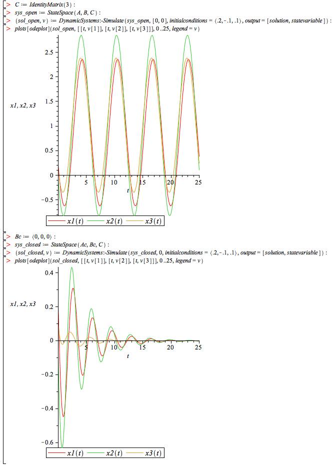
Increasing the computation precision, the solver successfully finds the LQR gain and the closed loop system is stable (all eigenvalues of the closed loop system have negative real parts).
We are now able to simulate the open-loop and closed-loop response of the system

If you have Maple 15, you can try the examples on this page yourself:
|
