New Features in Maple 15: Parametric Solving	Statistics

Maple 15 includes many new facilties for handling parametrized equations. Maple 15 makes it possible to get full solutions to parametric polynomial equations, showing all the different solutions in terms of the properties of the unknown parameters. The sum command also accepts a new 'parametric' option to give full case discussions involving parameters. With new commands in the RegularChains package, you can compute real solutions of polynomial systems involving inequalities and inequations, which again allows you to explore parametric solutions.

Solving parametric polynomial equations
Sums with parametric bounds
Polynomial systems involving inequalities and inequations


Solving Parametric Polynomial Equations
Maple 15 can find full solutions to parametric polynomial equations in terms of the properties of the unknown parameters. Finding such solutions is an extremely difficult problem. Maple 15 uses sophisticated algorithms from the Groebner and RegularChains packages in order to compute such answers.

You can ask for the full parametric solution to be returned:



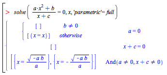
or you can ask for only the most general case to be returned, which is more computationally efficient. In that case, the remainder of the branches for the full answer is represented as an inert function call, so that the other solutions will be available to you later if needed.



You can expand this result into a full answer:



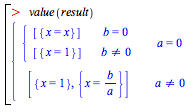
Here is a more complicated example, involving the equations for two ellipses of unknown radii:



Solving these two equations would give a general formula for the intersection of the two ellipses in terms the parameters r1, r2, q1, q2.



This is a generic solution, which is valid for most values of the parameters.



Here all the solutions are real, so you can plot what is happening:



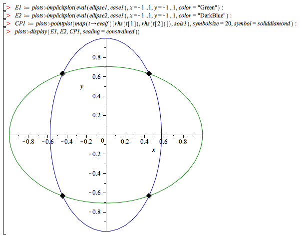
However, a generic solution may not be valid for all parameter values. This happens, for example when the ellipses do not intersect:



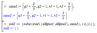
There is no solution, so clearly the generic solution that you computed earlier is not valid for this choice of parameters.

The plot below shows that the ellipses do not intersect in the real plane (in fact there are no complex intersections either).



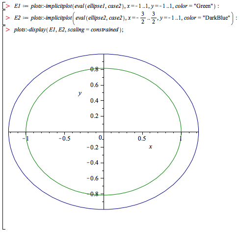
The new functionality in solve allows you to generate solutions which specialize better by using the 'parametric' option.



This new solution, while larger, will specialize properly in both cases:



For reasons of size and efficiency, solve parametric computes the explicit solution only in the generic case. So, in the second case, it does not provide an explicit answer, but instead it gives an inert answer which produces a solution when the command value is called on it.



This confirms that there are no real or complex solutions for this particular choice of parameters.

Sums with Parametric Bounds
The sum command was also extended with a new parametric option. When this option is specified, sum returns a piecewise case discussion for definite sums with parametric bounds.

For example:



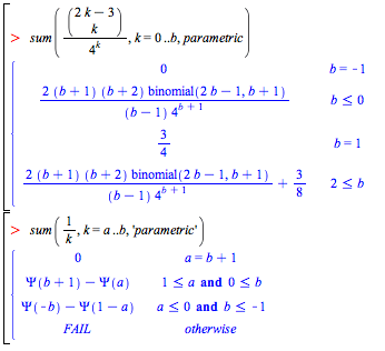
This next example shows that it is not always possible to return any solution, unless you distinguish between parametric cases:



The algorithm behind this first computes the indefinite sum of the argument, using one of the methods described in sum[details]. Then it finds the singularities of both the argument and its indefinite sum. This is done using the new option failpoints that was added to the indefinite summation commands SumTools[IndefiniteSum][Indefinite], SumTools[IndefiniteSum][Hypergeometric], and SumTools[IndefiniteSum][Rational]. Finally, correction terms and the corresponding parametric conditions are determined.

For example, consider the sum above:



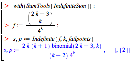
This indicates that the indefinite sum s has a singularity at k = 2, in this case a removable one:



Note, however, that the discrete summability condition

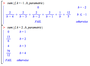
does not hold when the summation interval contains the singularity, i.e., when a ≤ 2 and 2 ≤ b:



The difference is exactly the correction term seen in the parametric result above.

Consider another example:



The first component of p lists all the intervals where f is singular, namely, for k ∈ {0, 1, 5}). The second component lists all the points where
s is singular but f is not, namely, k = 2, 3, 4. In this case, the singularities are not removable.



Polynomial Systems Involving Inequalities and Inequations
Finally, there are some new features in the RegularChains package concerning parametric systems. These routines are more specialized but will often be used by high-level routines, such as solve. The three new commands RealTriangularize, LazyRealTriangularize, and SamplePoints deal with arbitrary semi-algebraic systems. That is, given any system S of polynomial equations, polynomial inequations and polynomial inequalities (strict or large) these commands produce information about the real solutions of this system.

RealTriangularize returns a full description of the real solutions of S: it computes simpler systems S₁, ... , S_e such that a point is a solution of S if and only if it is a solution of one of the systems S₁, ... , S_e. Each of these systems has a triangular shape and remarkable properties: for this reason it is called a regular semi-algebraic system and the set of the S₁, ... , S_e is called a full triangular decomposition of S.



Compute a triangular decomposition of the 4-variable hypersurface, this system defines:



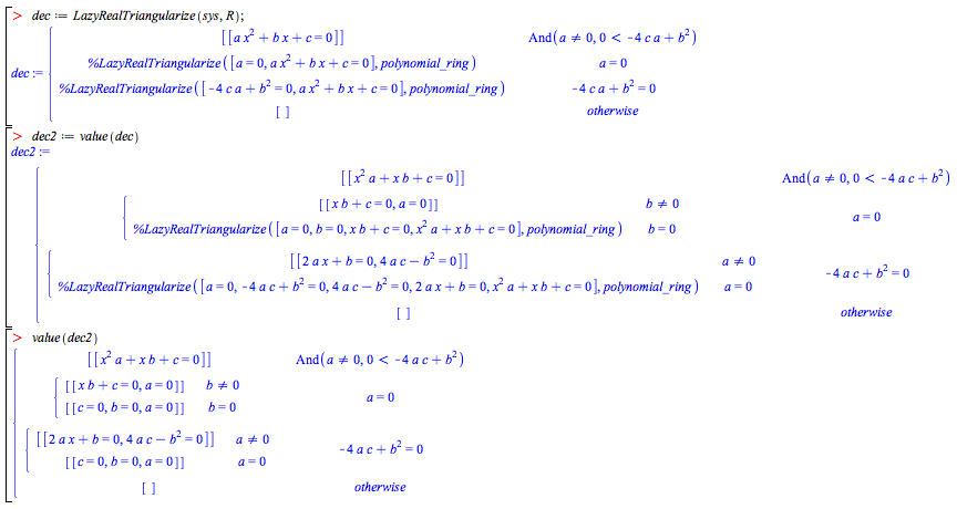
LazyRealTriangularize allows the user to compute a triangular decomposition of S in an interactive manner. This feature is particularly well adapted for systems that are hard to solve. For such systems, LazyRealTriangularize returns the components of S of maximum dimension together with unevaluated recursive calls, such that, when fully evaluated, these calls produce the other components of S (which are generally harder to compute).

Consider again the generic equation of degree two. Now, solve it interactively:




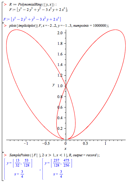
SamplePoints is an even a lazier (and thus much much more efficient) way of solving: it produces at least one sample point per connected component of the solution set of S. This way of solving is often sufficient in practical problems.

Consider again the generic equation of degree two and compute sample points of the 4-variable hypersurface it defines:



Now consider the Tacnode curve. Look for sample points in the middle of the right branch.

Statistics