Maple 17 is the result of many thousands of hours of work by world-class mathematicians at Maplesoft as well as experts in research labs and universities all around the world. Maple 17 offers numerous advancements in a variety of branches of mathematics that push the frontiers of mathematical knowledge and Maple’s capabilities.

In addition to the work done in group theory, statistics, physics, differential geometry, and more, Maple 17 also provides:

• Ground-breaking achievements in solving a whole new class of differential equations
• Major advancements in solving systems of equations, introducing new solution methods for systems of linear equations and  inequalities and for systems involving nonlinear polynomial inequalities
• New algorithms for finding limits of bivariate rational functions
• Advancements in working with algebraic curves
• Significant improvements in graph theory, including new algorithms and scalability improvements
• More functionality for handling and exploring branch cuts

Details and Examples

• Bivariate Limits
• Branch Cuts of Mathematical Expressions
• Differential Equations
• Graph Theory
• Intersecting Plane Curves
• Linear Inequality Solving
• Semialgebraic System Solving
• Solving Equations with Branch Cuts

Bivariate Limits

The limit command has been enhanced for the case of limits of bivariate rational functions. Many such limits that could not be determined previously are now computable. The new algorithm specifically handles the case where the function has an isolated singularity at the limit point.

In Maple 16, the following limit calls would return unevaluated, but they can be computed in Maple 17:

Example 1	Example 2	Example 3
>   >	>   >	>   >

Let us plot these three functions in the neighborhood of the origin:

>

>

>

In the last two examples, we can visually verify the existence of the limit.

In the first example, by inspecting the graph we can identify two different directions with different limits, namely and . Indeed:

>   >   >   >   >   >

How does Maple determine these limits? Let us consider a circle given by , where we will later let . Using the theory of Lagrange multipliers, the extremal values (maxima and minima) of the function  on the circle, for a fixed radius , satisfy the condition that the gradient of the function and the gradient of the constraint equation of the circle are parallel:

>

 

>

 

>

 

>

 

>

 

Thus, the maximal and minimal values of  on occur when both and For the bivariate limit, this means that it is sufficient to consider only those critical paths satisfying . In the example, there are two such paths, namely, and , and indeed they are exactly the same two paths from above leading to the extremal values and . Since we have found two directions with different limits, we can conclude that the bivariate limit does not exist.

The following graph depicts both critical paths in the -plane:

>

Note that the critical paths are not necessarily always lines. For example, in the second example above:

>   >   >

In fact, we can give nonlinear closed form expressions for the critical paths:

>

 

In our example, the limits along all of the critical paths are identical:

>

 

>

 

This is a proof that the bivariate limit of at the origin exists and is equal to .

The following graph depicts the function as well as all of the critical paths:

>   >

Branch Cuts of Mathematical Expressions

The FunctionAdvisor can now compute, algebraically, branch cuts (discontinuities) of mathematical expressions involving compositions of +, *, ^, and possibly fractional powers, with every mathematical function call for which FunctionAdvisor knows the branch cuts, with no restrictions to the level of nesting in the expression. This new feature includes the ability to generate 2-D and 3-D plots of the cuts, so as to view where the cuts are located and how the function evolves from one cut to another one.

Example

>   >   The segments of discontinuity are therefore located in the imaginary part of expression, . You can rotate these plots with the mouse and use any of the options of plot, plot3d and plotcompare to observe the cuts in different ways. A 2-D more abstract visualization of the same cuts: >

Example

A classic example in the theory of branch cut calculation: Kahan's teardrop >   This expression is equal to zero for all values of in the complex plane except for a small teardrop shaped region over the negative real axis, as shown in the following 3-D plot on the right (you can rotate it with the mouse). To see just the plot, without displaying the complicated algebraic description of the cuts, end the input with colon ':' >

Differential Equations

A new class of ordinary differential equations of Abel type, with non-constant invariants and depending on two arbitrary parameters, is now fully solvable in Maple 17.  Additionally, a large number of changes were added to the routines for tackling ordinary and partial differential equations.

Ordinary differential equation

For 1st order ODEs, the simplest problem beyond the reach of complete solving algorithms is known as Abel equations. These are equations of the form

where is the unknown and the and are arbitrary functions of . The biggest subclass of Abel equations known to be solvable was discovered by our research team and is the AIR 4-parameter class. New in Maple 17, another 2-parameter class of Abel equations, beyond the AIR class, is now known and solvable.

Example

>   >   >

The related class of Abel equations that is now entirely solvable consists of the set of equations that can be obtained from equation above by changing variables

where and the four are arbitrary rational functions of ; this is the most general rational transformation that preserves the form of Abel equations and thus generates Abel ODE classes.

Several changes were performed in the existing algorithms to optimize their functioning, resulting in new solutions for problems that were out of reach in previous releases.

Example: Second order linear equations

>   >   >

Example: Nonlinear ODE problems with initial values

>   >   >

Example: Third order nonlinear ODE depending on arbitrary function, a reduction to a Riccati equation

>   >   >

Partial differential equations

Changes were done in the existing algorithms for linear and nonlinear PDEs and systems of them, resulting in new solutions for more PDE problems.

Examples: Linear PDEs

>   >   Results can be verified with pdetest >   >   >   >   >   >   >

Examples: PDE problems with boundary conditions

>   >   >   The verification with pdetest also verifies that the solution satisfies the boundary conditions given >   Nonlinear PDE systems >   >   >

Graph Theory

Maple 17 has significant improvements to several GraphTheory commands, including:

• TuttePolynomial, ChromaticPolynomial, FlowPolynomial, AcyclicPolynomial and RankPolynomial
• IsIsomorphic

In addition, two new commands were added to the package:

• LaplacianMatrix
• ReliabilityPolynomial

Improvements to TuttePolynomial, ChromaticPolynomial, FlowPolynomial, AcyclicPolynomial and RankPolynomial commands

The TuttePolynomial command uses a new algorithm that is faster and consumes less memory.

For example, computation of the Tutte polynomial of the 12 vertex complete graph (CompleteGraph(12)) now requires 1/3 the memory, and completes in 1/3 the time.

For the 9,3 generalized Petersen graph (PetersenGraph(9,3)) the memory usage has dropped to 1/6, and the time to 1/8 of the time needed in Maple 16.

>

 

>

 

Example

>   >   memory used=106.98MiB, alloc change=0 bytes, cpu time=2.67s, real time=2.83s >   >   memory used=3.21MiB, alloc change=0 bytes, cpu time=125.00ms, real time=149.00ms

These improvements propagate to the commands ChromaticPolynomial, FlowPolynomial, AcyclicPolynomial and RankPolynomial as well.

Improvements to IsIsomorphic command

The IsIsomorphic command now utilizes a new algorithm that scales better to larger problems. As an example, two isomorphic soccer ball graphs (SpecialGraphs[SoccerBallGraph]) with 60 vertices and 90 edges can be tested for isomorphism in less than one second in Maple 17, while in Maple 16 and earlier, this same computation did not complete in under 10 minutes.

Example

>   >   >   >   memory used=448.29KiB, alloc change=0 bytes, cpu time=47.00ms, real time=50.00ms

The LaplacianMatrix command

The new LaplacianMatrix command can be used to compute the Laplacian matrix representation of a graph:

Example

>   >

The ReliabilityPolynomial command

The new ReliabilityPolynomial command can be used to compute the reliability polynomial of a graph:

Example

>

Intersecting Plane Curves

For Maple17, a new command, intersectcurves, has been added to the algcurves package.

>

 

Example
Given two plane curves expressed as polynomials in two variables: >   >   The intersectcurves command computes the points of intersection along with their multiplicities. Each set of intersection points is expressed as a list containing three values. The first two are irreducible polynomials, the second of which is in only one of the variables. The third value is either 0 or 1. When 1, the point is affine; when 0 it is a point in the projective plane (at infinity). >   This is to be interpreted as follows. There are two intersection points of multiplicity 2, namely, (-1,0) and (1,0), indicating that they are points where the curves intersect tangentially. In addition, there are two intersection points of multiplicity 1, namely, and . We can see all intersection points graphically with a simple implicit plot. >   >
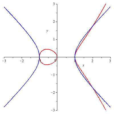
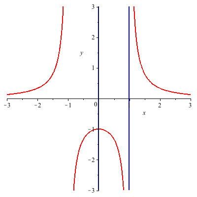
The following example illustrates the case when there are intersection points at infinity. >   >   >   >
There is one affine intersection point (0,-1) of multiplicity 1, plus one intersection point at infinity, of multiplicity 5. The tangent at this point is the line . Each of the two blue vertical lines intersects each of the two asymptotes of the red curve at the infinite point All but one of these intersections have multiplicity 1, and the exceptional one, between the blue line and the asymptote to the red curve at , comes from a tangential intersection, of multiplicity 2. 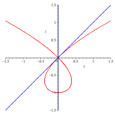We can perform a change of coordinates in order to plot this in the affine plane. First, we homogenize the equations, introducing a third variable , and then we substitute in order to move the intersection point that was previously at infinity to the origin. >   >   >   >   After the coordinate transformation, all intersection points (of and ) are visible in the plot and there are no intersection points at infinity.

Linear Inequality Solving

The LinearSolve command in the RegularChains package, whose purpose is to solve systems of linear equations and inequalities, has been enhanced in several ways:

• A more efficient algorithm based on Fourier-Motzkin elimination, has been implemented.
• Two new options, canonical and projection, for controlling the form of the output have been added.

The examples below illustrate the use of this command and the two new options for computations with polyhedra.

Change of representation for polyhedra

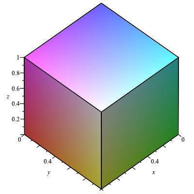
There are at least two ways to mathematically describe a polyhedron, either by specifying its corners, or by specifying its bounding hyperplanes. We start by illustrating this using a cube of side length 1 with one corner at the origin and its three adjacent edges parallel to the three coordinate axes.

Example
Plot the cube: >   >
Define this cube by bounding planes: >   Alternatively, define the vertices of the same cube: >   Suppose now that we are given the vertex representation and want to automatically derive the bounding planes representation. The cube is defined as the convex hull of all its vertices: >   >   >   >   >   We can now use the LinearSolve command to eliminate all from this system of equations and inequalities. We use the projection option to specify that elimination is required, and the canonical option to eliminate redundant equations and inequalities. >   >   >   This agrees with the representation above.

Dual polyhedra

Example
For every convex 3-D polyhedron, there is a dual polyhedron with the roles of corners and faces swapped. Let us compute the dual polyhedron of the cube. We start with a representation of the cube with the origin as the center. >   Now we rewrite this in matrix form. >   >   >   >   In general, if a bounded convex polyhedron is given by a set of inequalities of the form , then the vertices of its dual are exactly the columns of the matrix . The convex hull of these six vertices defines an octahedron. Using the same method as before, we compute the bounding planes for this octahedron. 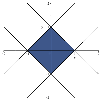>   >   >   >   >   >   >   The first two inequalities represent that projection of the octahedron onto the axis: >   Together with the following four inequalities, which involve only and but not , this defines the projection of the octahedron onto the -plane: >
The following plot shows this projection (blue) together with the four boundary lines. >
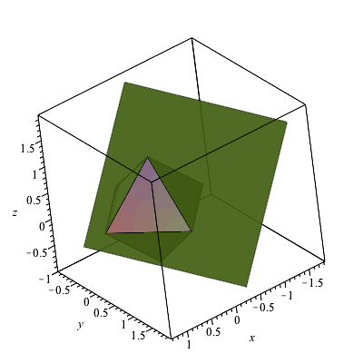
Finally, the last 8 inequalities, i.e., the ones containing , define the bounding planes of the octahedron. >   The following 3-D plot displays the tetrahedron as well as the last of these 8 bounding planes. Rotate the plot with the mouse in order to see that the plane actually touches one of the faces. >   >

Semialgebraic System Solving

The SolveTools[SemiAlgebraic] command has been integrated directly into the solve command, such that many systems involving non-linear polynomial inequalities that could not be solved previously, are solved.

In Maple 16, no solutions were found for the following system, but in Maple 17 it is easily solved:

Example
>
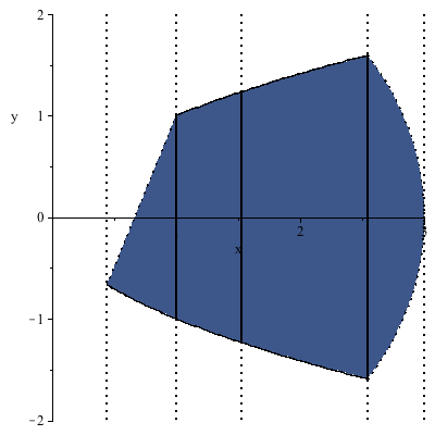
A solution to such a system of inequalities is a decomposition of the feasible region of the inequalities into bands as can be seen in the inequality plot: >
Additionally, the SemiAlgebraic command now can build case discussions for systems with real-valued parameters. >

Solving Equations with Branch Cuts

New functionality has been added to the solve command to account for branch cuts in the input equations and build piecewise expressions that are correct for substitution of parameters. This functionality is controlled with the new option symbolic = false;. The default behavior in Maple 17 and previous versions of Maple, is the same as specifying symbolic = true;.

Example

>   >   >   While both sol1 and sol2 are valid for some values of the parameter : >   Only the solution using the option are valid for other values of the parameter: >