With every new release, Maplesoft strives to improve the efficiency and speed of its mathematical computations. This involves making improvements in the most frequently called routines and algorithms, as well as in the low-level infrastructure.

• New algorithms result in faster calculations with complex floating-point numbers, with some calculations up to 2000 times faster.
• Performance enhancements for floating-point linear algebra operations include improved use of multiple cores and CPUs as well as faster operations with sparse vectors and matrices.
• Memory usage in Maple is much improved with the combination of multiple memory regions and parallel memory management. The use of multiple memory regions reduces fragmentation and makes much more efficient use of overall memory.
• Parallel memory management takes advantage of multiple processors to perform memory management tasks more quickly, resulting in a 10% reduction of running times on average, with memory-intensive computations running up to 50% faster. As a result of these improvements, you can solve bigger problems, get better performance for your computations, and have more available memory for other programs running on the same machine.
• Numerous improvements in underlying routines combined with a new high performance data structure for distributed multivariate polynomials drastically improves the speed and scalability of most polynomial computations.

Details and Examples

• Elementary Functions
• Multiple Memory Regions
• Parallel Linear Algebra
• Parallel Memory Management
• Polynomial Arithmetic
• Sparse Matrices and Vectors

Elementary Functions

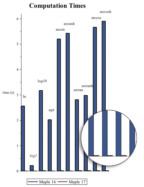
Hardware algorithms have been introduced into Maple 17 that greatly speed up operations on complex floating-point numbers. Compared to Maple 16, the Maple 17 is almost 2000 times faster in some cases.

To demonstrate this, the following commands create a random vector, V, containing 10,000 complex floating-point numbers. The time (in seconds) needed to perform operations on all 10,000 elements is found using various functions.

Example
Benchmarks computed on an Intel Q8200 2.33GHz Quad-Core CPU running Linux. >   >     >     >   >   >   >   >   >   >   >   The following lists, m16 and m17, contain the measured times to compute these operations using Maple 16 and 17, respectively. The column graph plots these lists to show the speed up between the two versions. >   >   >

Multiple Memory Regions

A significant improvement to Maple's memory allocator is the addition of multiple memory regions.

Benefits of multiple memory regions include:

• More efficient allocation of memory, leading to more memory being available to solve bigger problems without the need to initially specify the size of the reserved region.
• Better resource sharing between different processes running on the same machine, including multiple cores of Maple and multiple Maple kernels launched as parallel nodes in a grid.
• Performance improvements due to less fragmentation and cache locality, as well as performance improvements when running parallel code.

Previously, Maple initially reserved a large contiguous heap of memory that was subsequently managed by additional allocations and garbage collection as required. Initially, only a small fraction of this reserved memory was allotted to handle memory allocation requests. Whenever a given allotment was exhausted, a garbage collection would occur to reclaim any unused memory. As the computation required more memory, the memory management system would progressively commit more of the heap to be allocated.With the addition of memory regions, Maple is no longer constrained by the limitation imposed by a single large contiguous memory region (heap).  Instead, Maple is able to incorporate additional regions upon demand. Various types of memory regions are provided: small allocations come from thread-local regions (512 words and less), medium-sized allocations reside in global thread-shared regions (less than 1MB), and finally large blocks of memory are individually allocated as distinct regions of their own. Overall, this allows Maple to more effectively and efficiently manage the available memory resources, and more specifically, this offers improvements to caching via better data locality and reduced fragmentation.In earlier releases of Maple, when a chunk of memory was committed, it remained under Maple's control for the remainder of the session. Handling memory requests larger than 1MB by allocating an individually tailored memory region enables Maple 17 to return this large block of memory back to the operating system when it is no longer needed.

Example

The following code snippet allocates a couple of large matrices, A and B, does some work, and then clobbers A and B, thereby rendering the allocated memory garbage.  Notice, that memory usage drops after the explicit call to garbage collection.* >   >   >   * The explicit call to gc() is used here to illustrate a specific behavior of Maple's memory management system. In general, it is better to allow Maple to decide when to initiate a garbage collection cycle.

Parallel Linear Algebra

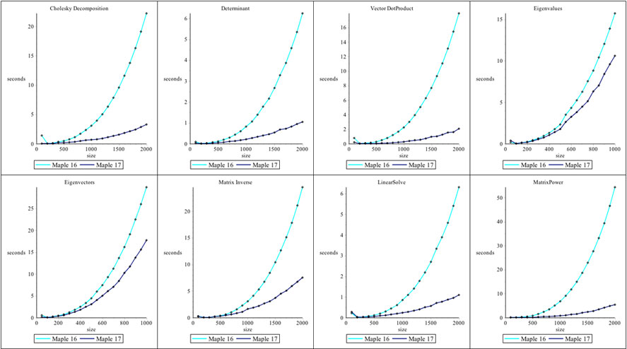
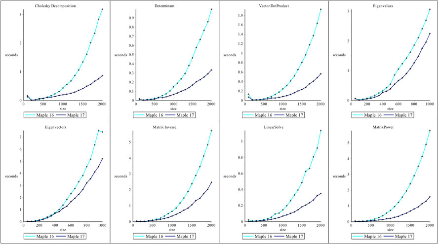
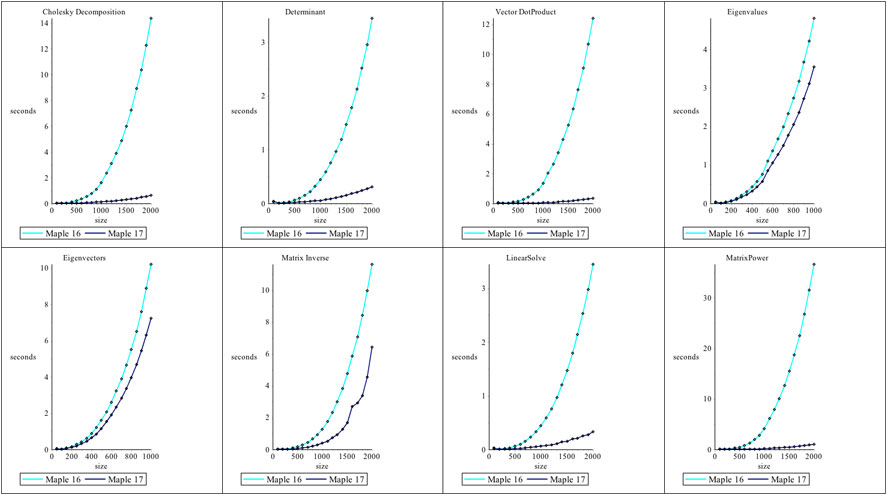
The access to optimized BLAS and LAPACK functions for floating-point Matrices and Vectors has been updated in Maple 17.On Linux and OS X, this involves updates to the ATLAS (Automatically Tuned Linear Algebra Software) dynamic libraries which are shipped with Maple.  While on 64-bit Windows, Maple 17 has been updated to use Intel's Math Kernel Library (MKL).  Performance enhancements for floating-point Linear Algebra operations include improved use of multiple cores and CPUs.The operations referenced in the plots in this document were all performed on real, floating-point Matrices and Vectors created with the datatype=float[8] option.

Linux (32bit)

Linux (64bit)

OS X

Windows (64bit)

Parallel Memory Management

One of the core components of Maple's engine is the 'garbage collector'. The garbage collector is responsible for finding and reclaiming memory that is no longer needed by the evaluation engine. In Maple 17, the garbage collector is capable of taking advantage of multiple processors to perform its job more quickly. As the garbage collector is used continuously as Maple runs, this speed up helps all users, not just those running parallel algorithms.

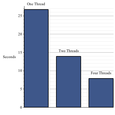
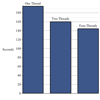
• The garbage collector in Maple 17 is capable of running multiple threads to take advantage of multiple cores.  This can speed up the collector significantly.  Although the collector is only responsible for a fraction of Maple's total running time, this can still lead to running times reduced by 10% on average, with memory-intensive computations running up to 50% faster.  These speed ups require no changes to user code.There are 2 kernelopts that can control the parallel collector.gcmaxthreads controls the maximum number of threads that the parallel garbage collector will use.gcthreadmemorysize controls how many threads Maple will use for a collection.  The number of bytes allocated is divided by the value assigned to gcthreadmemorysize to determine the number of threads.

Example
The following example shows the speed up in the garbage collector from using multiple threads. >   >   >   >   >   >   >   >
Of course, the average compuation does not require such intensive memory management, so the garbage collection algorithm only comprises a small amount of the total Maple running time. But even in this more typical example, the improvement is significant. >   >   >   >   >    >   >    >   >    >

Polynomials with Integer Coefficients

Maple 17 automatically uses a new high performance data structure for distributed multivariate polynomials with integer coefficients.  Together with new algorithms in the Maple kernel, this drastically improves the speed and scalability of most polynomial computations.  

Benchmarks computed in real times on a 64-bit quad core Intel Core i7 920 2.66 GHz.

Overview

Expanding this polynomial with 170544 terms takes 31 milliseconds and 2.6 MB of memory in Maple 17, versus 250 ms and 29 MB in Maple 16. This speedup is entirely due to the reduction in overhead for the new data structure. The external C routine that computes this result has not changed. >   >   Maple 17: memory used=2.67MiB, alloc change=2.61MiB, cpu time=30.00ms, real time=31.00ms Maple 16: memory used=23.40MiB, alloc change=29.16MiB, cpu time=242.00ms, real time=250.00ms Mathematica® 9: 0.564 seconds AbsoluteTiming[ f = Expand[ (1+x+y+z+t+u+v+w)^15 ]; ]
Common queries such as finding the variables, computing the total degree, and testing for a polynomial run in O(1) time for the new data structure.  The effect on Maple library is profound. >   >   >   Maple 17: memory used=0.59KiB, alloc change=0 bytes, cpu time=0ns, real time=0ns memory used=0.59KiB, alloc change=0 bytes, cpu time=0ns, real time=0ns memory used=432 bytes, alloc change=0 bytes, cpu time=0ns, real time=0ns Maple 16: memory used=0.66KiB, alloc change=0 bytes, cpu time=76.00ms, real time=77.00ms memory used=0.72KiB, alloc change=0 bytes, cpu time=119.00ms, real time=119.00ms memory used=0.55KiB, alloc change=0 bytes, cpu time=53.00ms, real time=54.00ms Mathematica® 9: 0.125 seconds, X = Variables[ f ] 0.166 seconds, d = Exponent[ f, x]  (* degree in x, total degree not builtin *) 4.611 seconds, PolynomialQ[ f ]
New high performance algorithms were developed for the Maple kernel to exploit the new data structure.  We improved many core operations including differentiation, extracting a coefficient, and evaluating a polynomial. >   >   >   Maple 17: memory used=2.60MiB, alloc change=2.61MiB, cpu time=5.00ms, real time=5.00ms memory used=5.21MiB, alloc change=2.61MiB, cpu time=21.00ms, real time=21.00ms memory used=2.60MiB, alloc change=2.61MiB, cpu time=26.00ms, real time=26.00ms Maple 16: memory used=12.36MiB, alloc change=9.72MiB, cpu time=174.00ms, real time=175.00ms memory used=34.78MiB, alloc change=29.16MiB, cpu time=194.00ms, real time=194.00ms memory used=48.63MiB, alloc change=34.02MiB, cpu time=476.00ms, real time=478.00ms Mathematica® 9: 1.001 seconds, D[f,x]; 1.030 seconds, CoefficientList[f, x]; 1.304 seconds, f /. {x->2, y->3, z->5};
Dense methods have been added to multiply multivariate polynomials in subquadratic time.  Maple 17 automatically selects a sparse or dense algorithm, balancing time and memory use.   >   >   Maple 17: memory used=2.55MiB, alloc change=0.61MiB, cpu time=148.00ms, real time=149.00ms Maple 16: memory used=4.07MiB, alloc change=0 bytes, cpu time=4.55s, real time=1.19s Mathematica® 9: 1.331 seconds g = Expand[ (x^5+x^3+x^2+x+1)^20 (y^5+y^3+y^2+y+1)^20 ]; AbsoluteTiming[ p = Expand[ (g+1)*(g+2) ]; ]
Parallel speedup increases in Maple 17 due to the elimination of sequential overhead and Amdahl's Law.  For the factorization below, Maple 17 uses 26.01 CPU seconds versus 62.24 for Maple 16, so it saves a little more than half the work.  However, all of the time saved was sequential, so Maple 17 actually runs 3.7x faster on the quad core CPU, and parallel speedup increases from 1.3x to 2.0x. >   >   >   Maple 17: memory used=1.43GiB, alloc change=82.04MiB, cpu time=26.01s, real time=12.90s Maple 16: memory used=4.29GiB, alloc change=256.41MiB, cpu time=62.24s, real time=47.60s Mathematica® 9: 952.857 seconds f = Expand[ (1+x+y+z+t)^20 ]; p = Expand[ (f+1)*(f+2) ]; AbsoluteTiming[ Factor[ p ]; ]

Benchmarks

For each problem we expand the input and , then we time the multiplication , the division , and the factorization of .

For Maple we timed p := expand(f*g); divide(p,f,'q'); and factor(p);

For Mathematica® we timed p = Expand[f g]; PolynomialQuotient[p, f, x]; and Factor[p]; except for Problem #5 where Cancel[p/f]; was much faster than PolynomialQuotient.

All times are real times in seconds on a 64-bit Core i7 920 2.66GHz Linux system.

Problem #1:   1771 x 1771 = 12341 terms	Problem #2:   1771 x 1771 = 12341 terms	Problem #3:   5456 x 5456 = 39711 terms
Problem #4:   10626 x 10626 = 135751 terms	Problem #5:   9261 x 9261 = 12552 terms	Problem #6:   3003 x 3003 = 417311 terms

The timing data is given in matrix form below.  Mathematica® 9 is the first row, Maple 16 is the middle row, and Maple 17 is the last row.

Sparse Matrices and Vectors

Enhancements have been made in Maple 17 for the performance of stacking and augmenting sparse floating-point, hardware datatype Matrices and Vectors. Computing linear combinations of pairs of sparse floating-point, hardware datatype Matrices using the LinearAlgebra:-MatrixAdd command has also been improved.In the examples below, the Matrix and Vector constructors are used for stacking or augmentation (concatenation).Benchmarks computed in 64-bit Maple 17 for Linux on an Intel Core i5 CPU 760 @ 2.80GHz.

Sparse vector concatenation

In Maple 16, the concatenation of Vector V with itself three times would take approximately 28 seconds and would result in an output Vector with full rectangular storage. The allocated memory would increase by 1.27GiB.

In Maple 17, it takes less than 0.2 seconds and produces a Vector with sparse storage. Memory allocation increases by 30.5MiB.

Example

>   >   >   >   >   memory used=76.37MiB, alloc change=30.54MiB, cpu time=100.00ms, real time=121.00ms >

Sparse matrix concatenation

In Maple 16, the concatenation of Matrix M with itself as performed below would take approximately 20 seconds and would result in an output Matrix with full rectangular storage.

In Maple 17, it takes less than 0.1 seconds and produces a Matrix with sparse storage. Memory allocation increases by 48MiB.

Example

>   >   >   >     >     memory used=0.76MiB, alloc change=48.00MiB, cpu time=30.00ms, real time=55.00ms   >

Simple linear combinations of sparse matrices

In Maple 16, the following command would take 3 minutes and allocated memory would increase by 400MiB.

In Maple 17, it takes less than 1 second and allocated memory increases by 76MiB.

Example

>   >   >   >   memory used=76.67MiB, alloc change=76.35MiB, cpu time=360.00ms, real time=417.00ms

---

Signal Processing